Introduction to the YOLO Family

---

---

Introduction to the YOLO Family

Object detection is one of the most crucial subjects in computer vision. Most computer vision problems involve detecting visual object categories like pedestrians, cars, buses, faces, etc. It is one such field that is not just limited to academia but has a potential real-world business use case in domains like video surveillance, healthcare, in-vehicle sensing, and autonomous driving.

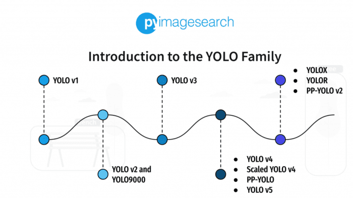
Many use cases, especially autonomous driving, require high accuracy and real-time inference speed. Hence, choosing an Object Detector that fits the bill for both speed and accuracy becomes essential. YOLO (You Only Look Once) is a single-stage object detector introduced to achieve both goals (i.e., speed and accuracy). And today, we will give an introduction to the YOLO family by covering all the YOLO variants (e.g., YOLOv1, YOLOv2,…, YOLOX, YOLOR).

Since its inception, the object detection field has grown significantly, and the state-of-the-art architectures generalize pretty well on various test datasets. But to understand the magic behind these current best architectures, it is necessary to know how it all started and how far we have reached in the YOLO family.

There are three classes of algorithms in object detection:

• Based on Traditional Computer Vision
• Two-Stage Deep Learning based algorithms
• The third one is Single-Stage Deep Learning based algorithms

And today, we are going to discuss the YOLO object detection family, which falls under the Single-Stage Deep Learning algorithms.

We believe that this is a one-of-a-kind blog post covering all the YOLO variants in one post and would help you get a great insight into each variant and might help you select the best YOLO version for your project.

This lesson is the first tutorial in our 7-part series on the YOLO Object Detector:

1. Introduction to the YOLO Family (this tutorial)
2. Understanding a Real-Time Object Detection Network: You Only Look Once (YOLOv1)
3. A Better, Faster, and Stronger Object Detector (YOLOv2)
4. Mean Average Precision (mAP) Using the COCO Evaluator
5. An Incremental Improvement with Darknet-53 and Multi-Scale Predictions (YOLOv3)
6. Achieving Optimal Speed and Accuracy in Object Detection (YOLOv4)
7. Training the YOLOv5 Object Detector on a Custom Dataset

To learn how the YOLO family evolved with each variant different and better than the previous version in detecting objects in images, just keep reading.

---

Introduction to Object Detection

Recall in Image Classification the goal is to answer the question of “what is present in the image?” where the model attempts to comprehend the entire image by assigning the image with a specific label.

Generally, we deal with scenarios where only one object is present in the image classification. As shown in Figure 1, we have a Santa Claus and a few more objects, but the main object is Santa which is correctly classified with 98% probability. That’s great. In certain cases like this one, when an image depicts a single object, classification is enough to answer our question.

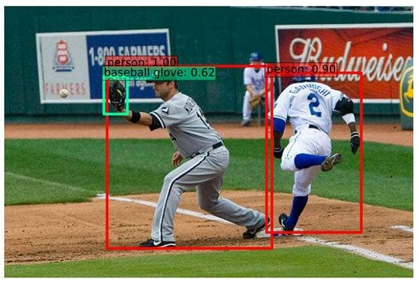
However, there are many scenarios when we cannot say what’s in the image with a single label, and image classification is not enough to help answer this question. For example, consider Figure 2, in which the model detects three objects: two persons and one baseball glove, and not just that, it also identifies the location of each object. This is known as object detection.

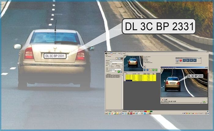
Another critical use case of object detection is Automatic License Plate Recognition, as shown in Figure 3. Now ask yourself a question, how would you recognize the alphabets and numbers of a car number plate unless you know the location of the number plate? Of course, first, you need to identify the location of the number plate with an object detector and then apply a second algorithm to recognize the digits.

Object detection involves both classification and localization tasks and is used to analyze more realistic cases in which multiple objects may exist in an image. Hence, object detection is a two-step process; the first step is finding the locations of objects.

And the second step is classifying these bounding boxes into different classes because this object detection suffers from all the problems associated with image classification. In addition, it has its challenges of localization and speed of execution.

---

Challenges

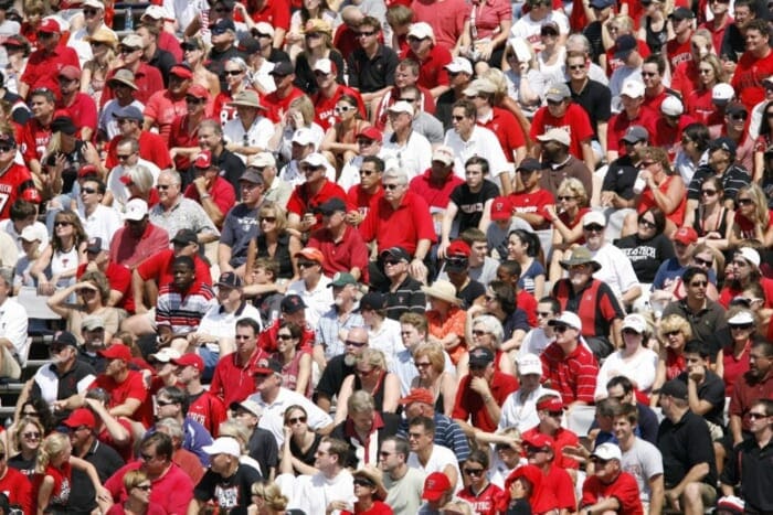
• Crowded or Cluttered Scenario: Too many objects in the image (Figure 4) make it extremely crowded. This creates various challenges for the object detect model, like the occlusions could be large, the objects could be small, and the scale could be inconsistent.

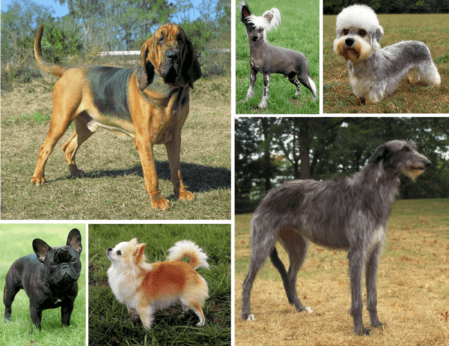
• Intra-Class Variance: Another major challenge for object detection is to correctly detect objects of the same class, which can have high variance. For example, as shown in Figure 5, there are six breeds of dogs, and all of them have different sizes, colors, fur length, ears, etc., so detecting these objects of the same class can be challenging.

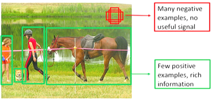
• Class Imbalance: It is a challenge that impacts almost all the modalities, be it an image, text, time-series; more specifically, in the image domain, image classification struggles a lot, and object detection is no exception. We call it a foreground-background class imbalance in object detection, as shown in Figure 6.
  
  To understand how class imbalance could pose a problem in object detection, consider an image containing very few primary objects. The remainder of the image is filled with the background. As a result, the model would look at many regions in the image (dataset) where most regions would be considered negatives. Because of these negatives, the model learns no useful information and can overwhelm the entire training of the model.

Many other challenges are associated with object detection like occlusion, deformation, viewpoint variation, illumination conditions, and essential speed for real-time detection (required in many industrial applications).

---

History of Object Detection

Object detection is one of the most critical and challenging problems in computer vision, and it has created a history in the past decade with its development. Nevertheless, the progress in this domain has been significant; every year, the research community achieves a new state-of-the-art benchmark. And of course, all of this wouldn’t have been possible without the power of Deep Neural Networks and the massive compute by NVIDIA GPUs.

In the history of object detection, there have been two distinct eras:

1. The traditional computer vision approaches were in the game until 2010,
2. From 2012, a new era of convolutional neural networks started when AlexNet (an image classification network) won the ImageNet Visual Recognition challenge.

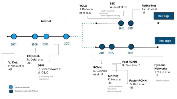
This distinction between the two eras is also evident in Figure 7, which shows the roadmap of object detection, starting with the Viola–Jones Detector in 2004 to EfficientDet in 2019. It is worth mentioning that the Deep-Learning-based detection methods are further classified into two-stage detectors and single-stage detectors.

Most traditional object detection algorithms like Viola–Jones, Histogram of Oriented Gradients (HOG), and Deformable Parts Model (DPM) relied on extracting handcrafted features like edges, corners, gradients from the image and classical machine learning algorithms. For example, The Viola–Jones, a first object detector, was only designed to detect frontal faces of humans and did not do well on sideways and up/down faces.

Then, in 2012 came a new era. A revolution that changed the game for computer vision entirely when AlexNet, a Deep Convolutional Neural Network (CNN) architecture, was born out of the need to improve the results of the ImageNet challenge achieved considerable accuracy on the 2012 ImageNet LSVRC-2012 challenge with an accuracy of 84.7% as compared to the second-best with an accuracy of 73.8%.

Then it was just a matter of time before these state-of-the-art image classification architectures started being used as a feature extractor in the object detection pipeline. Both problems are interrelated, and they rely on learning robust high-level features. Hence, Girschick et al. (2014) showed how we could use convolutional features for object detection, introducing R-CNN (applying CNN on region proposals). Since then, object detection has started to evolve at an unprecedented speed.

As shown in Figure 7, deep learning detection methods can be grouped in two stages; the first is called two-stage detection algorithms, making predictions at multiple stages, including networks like RCNN, Fast-RCNN Faster-RCNN, etc.

The second class of detectors is called single-stage detectors like SSD, YOLO, EfficientDet, etc.

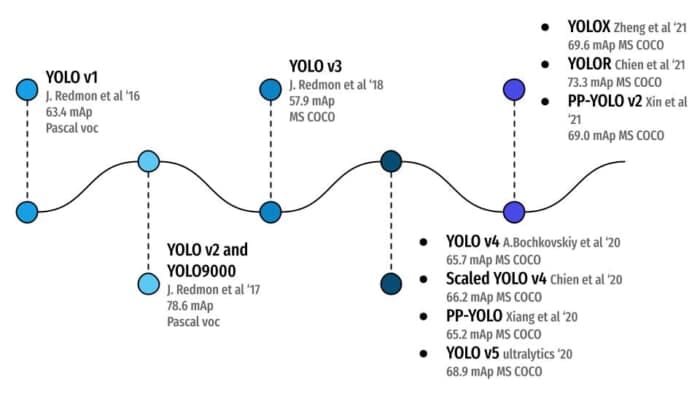
In Figure 8, you can see all the YOLO object detection algorithms and how they evolved, starting from YOLOv1 in the year 2016 achieving 63.4mAP on Pascal VOC (20 classes) dataset to YOLOR in the year 2021 with 73.3 mAP on much more challenging MS COCO dataset (80 classes). And that’s the beauty of academia. With continuous hard work and resilience, YOLO object detection has come a long way!

---

What Are Single-Stage Object Detectors?

Single-Stage Object Detectors are a class of object detection architectures that are one-stage. They treat object detection as a simple regression problem. For example, the input image fed to the network directly outputs the class probabilities and bounding box coordinates.

These models skip the region proposal stage, also known as Region Proposal Network, which is generally part of Two-Stage Object Detectors that are areas of the image that could contain an object.

Figure 9 shows the single-stage and two-stage detector workflow. In single-stage, we apply the detection head directly on the feature map, while, in two-stage, we first apply a region-proposal network on the feature maps.

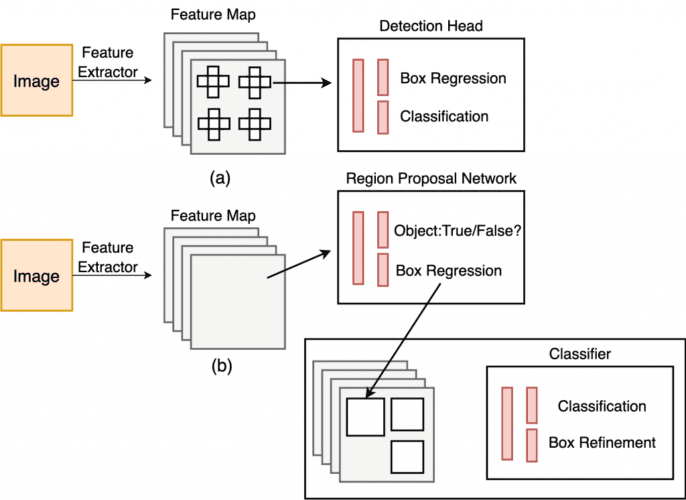
Then, these regions are further passed to the second stage, making predictions for each region. Faster-RCNN and Mask-RCNN are some of the most popular two-stage object detectors.

While two-stage detectors are considered more accurate than single-stage object detectors, they have a slower inference speed involving multiple stages. On the other hand, single-stage detectors are much faster than two-stage detectors.

---

YOLOv1

In 2016 Joseph Redmon et al. published the first single-stage object detector, You Only Look Once: Unified, Real-Time Object Detection, at the CVPR conference.

YOLO (you only look once) was a breakthrough in the object detection field as it was the first single-stage object detector approach that treated detection as a regression problem. The detection architecture only looked once at the image to predict the location of the objects and their class labels.

Unlike the two-stage detector approach (Fast RCNN, Faster RCNN), YOLOv1 does not have a proposal generator and refine stages; it uses a single neural network that predicts class probabilities and bounding box coordinates from an entire image in one pass. It can be optimized end-to-end since the detection pipeline is essentially one network; think of it as an image classification network.

Since the network is designed to train in an end-to-end fashion similar to image classification, the architecture is extremely fast, and the base YOLO model predicts images at 45 FPS (Frames Per Second) benchmarked on a Titan X GPU. The authors also came up with a much lighter version of YOLO called Fast YOLO, having fewer layers that process images at 155 FPS. Isn’t that amazing?

YOLO achieved 63.4 mAP (mean average precision), as shown in Table 1, more than double the other real-time detectors, making it even more special. We can see that both the YOLO and Fast YOLO outperforms the real-time object detector variants of DPM by a considerable margin in terms of mean average precision (nearly 2x) and FPS.

The generalizability of YOLO was tested on artwork and natural images from the internet. Furthermore, it considerably outperformed detection methods like the Deformable Parts Model (DPM) and Region-Based Convolutional Neural Networks (RCNN).

In our upcoming Lesson #2, we will do a deep-dive into YOLOv1, so do check that out!

---

YOLOv2

Redmon and Farhadi (2017) published the YOLO9000: Better, Faster, Stronger paper at the CVPR conference. The authors proposed two state-of-the-art YOLO variants in this paper: YOLOv2 and YOLO9000; both were identical but differed in training strategy.

YOLOv2 was trained on detection datasets like Pascal VOC and MS COCO. At the same time, the YOLO9000 was designed to predict more than 9000 different object categories by jointly training it on the MS COCO and ImageNet datasets.

The improved YOLOv2 model used various novel techniques to outperform state-of-the-art methods like Faster-RCNN and SSD in both speed and accuracy. One such technique was multi-scale training that allowed the network to predict at varying input sizes, thus allowing a trade-off between speed and accuracy.

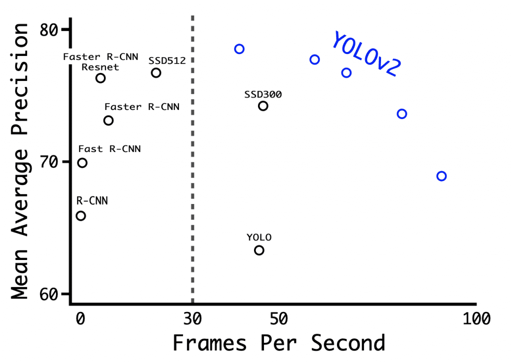
At 416×416 input resolution, YOLOv2 achieved 76.8 mAP on VOC 2007 dataset and 67 FPS on Titan X GPU. On the same dataset with 544×544 input, YOLOv2 attained 78.6 mAP and 40 FPS.

Figure 10 shows the benchmark of YOLOv2 on various resolutions on a Titan X GPU along with other detection architectures like Faster R-CNN, YOLOv1, SSD. We can observe that almost all the YOLOv2 variants perform better in speed or accuracy than the other detection frameworks, and a sharp trade-off between accuracy (mAP) and FPS can be observed in YOLOv2.

For a detailed review on YOLOv2, watch for our upcoming Lesson #3.

---

YOLOv3

Redmon and Farhadi (2018) published the YOLOv3: An Incremental Improvement paper on arXiv. The authors made many design changes concerning the network architecture and adapted most of the other techniques from YOLOv1 and especially YOLOv2.

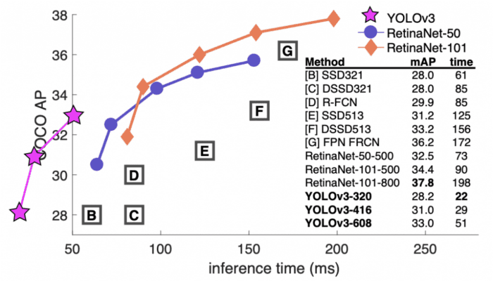
This paper introduced a new network architecture called Darknet-53. The Darknet-53 is a much bigger network than before and is much more accurate and faster. It is trained at various image resolutions like 320×320, 416×416. At the 320×320 resolution, YOLOv3 achieves 28.2 mAP runs at 45 FPS on the Titan X GPU and is as accurate as Single-Shot Detector (SSD321) but 3x faster (shown in Figure 11).

We break down YOLOv3 completely in our upcoming Lesson #5.

---

YOLOv4

YOLOv4 is a product of many experiments and studies that combine various small novel techniques that improve the Convolutional Neural Network accuracy and speed.

This paper did extensive experiments across different GPU architectures and showed that YOLOv4 outperformed all the other object detection network architectures in terms of speed and accuracy.

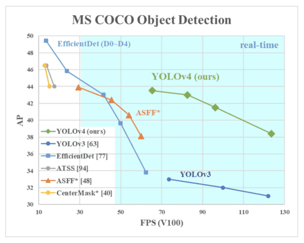
In 2020, Bochkovskiy et al. (the author of a renowned GitHub Repository: Darknet) published the YOLOv4: Optimal Speed and Accuracy of Object Detection paper on arXiv. We can observe from Figure 12 that YOLOv4 runs twice faster than EfficientDet with comparable performance, and it improves YOLOv3’s mAP and FPS by 10% and 12%.

Convolutional Neural Network (CNN) performance depends greatly on the features we use and combine. For example, some features work only on a specific model, problem statement, and dataset. But features like batch normalization and residual connections apply to most models, tasks, and datasets. Thus, these features can be called universal.

Bochkovskiy et al. leverage this idea and assume a few universal features, including

• Weighted-Residual-Connections (WRC)
• Cross Stage Partial connections (CSP)
• Cross mini-Batch Normalization (CmBN)
• Self-adversarial training (SAT)
• Mish activation
• Mosaic data augmentation
• DropBlock regularization
• CIoU loss

The above features are combined to achieve state-of-the-art results: 43.5% mAP (65.7% mAP50) on the MS COCO dataset at a real-time speed of ∼65 FPS on the Tesla V100 GPU.

The YOLOv4 model combined the above and more features to form “Bag of Freebies” for improving the training of the model and “Bag-of-Specials” for improving the accuracy of the object detector.

We cover YOLOv4 comprehensively with code in our upcoming Lesson #6.

---

YOLOv5

In 2020, after the release of YOLOv4, within just two months of period, Glenn Jocher, the founder and CEO of Ultralytics, released its open-source implementation of YOLOv5 on GitHub. YOLOv5 offers a family of object detection architectures pre-trained on the MS COCO dataset. It was followed by the release of EfficientDet and YOLOv4. This is the only YOLO object detector that does not have a research paper which initially led to some controversies; however, soon, that notion was broken as its capabilities undermined the noises.

Today, YOLOv5 is one of the official state-of-the-art models with tremendous support and is easier to use in production. The best part is that YOLOv5 is natively implemented in PyTorch, eliminating the Darknet framework’s limitations (based on C programming language and not built with production environments perspective). Darknet framework has evolved over time and is a great research framework to work with, training, fine-tuning, inference with TensorRT; all of this is possible with Darknet. However, it has a smaller community and hence, less support.

This huge change of YOLO in PyTorch made it easier for the developers to modify the architecture and export to many deployment environments straightforwardly. And not to forget, YOLOv5 is one of the official state-of-the-art models hosted in the Torch Hub showcase.

As you can see in the below shell block, you can run an inference with YOLOv5 and PyTorch Hub in just five lines of code. Isn’t that amazing?

$ import torch
$ model = torch.hub.load('ultralytics/yolov5', 'yolov5s')  # or yolov5m, yolov5l
$ img = 'https://ultralytics.com/images/zidane.jpg'  # or file, Path, PIL, OpenCV
$ results = model(img)
$ results.print()  # or .show(), .save()

At the time of release, YOLOv5 was state of the art among all known YOLO implementations. Since the release of YOLOv5, the repository has been very active, with more than 90 contributors since the YOLOv5-v1.0 was released.

The YOLOv5 repository has tons to offer from a development perspective, making it so much easier to train, fine-tune, test, and deploy on various target platforms. Some of the out-of-the-box tutorials they offer include:

• Training on Custom Dataset
• Multi-GPU Training
• Exporting the trained YOLOv5 model on TensorRT, CoreML, ONNX, and TFLite
• Pruning the YOLOv5 architecture
• Deployment with TensorRT

Moreover, they have developed an iOS application called iDetection, which offers four variants of YOLOv5. We tested the application on iPhone 13 Pro, and the results were impressive; the model runs detection at close to 30FPS.

Same as YOLOv4, the YOLO v5 uses Cross-Stage Partial Connections with Darknet-53 in the Backbone and Path Aggregation Network as the Neck. The major improvements include novel mosaic data augmentation (from YOLOv3 PyTorch implementation) and auto-learning bounding box anchors.

---

Mosaic Data Augmentation

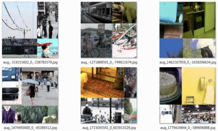
The idea of mosaic data augmentation was first used in the YOLOv3 PyTorch implementation by Glenn Jocher and is now used in YOLOv5. Mosaic augmentation stitches four training images into one image in specific ratios, as shown in Figure 13. Mosaic augmentation is especially useful for the popular COCO object detection benchmark, helping the model learn to address the well-known “small object problem” – where small objects are not as accurately detected as larger objects.

The benefit of using mosaic data augmentations is

• The network sees more context information within one image and even outside their normal context.
• Allows the model to learn how to identify objects at a smaller scale than usual.
• Batch normalization would have a 4x reduction because it will calculate activation statistics for four different images at each layer. This would reduce the need for a large mini-batch size during training.

---

Quantitative Benchmark

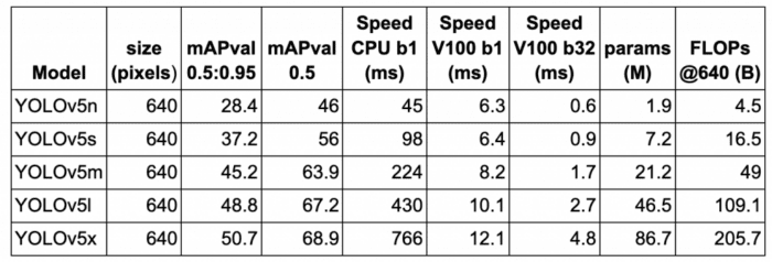
In Table 2, we show the performance (mAP) and speed (FPS) benchmarks of five YOLOv5 variants on the MS COCO validation dataset at 640×640 image resolution on Volta 100 GPU. All five models were trained on the MS COCO training dataset. The model benchmarks are shown in ascending order starting with YOLOv5n (i.e., the nano variant having the smallest model footprint to the largest model, YOLOv5x).

Consider YOLOv5l; it achieves an inference speed of 10.1ms (or 100 FPS) with batch size = 1 and 67.2 mAP at 0.5 IOU. In contrast, YOLOv4 with 608 resolution on V100 achieved an inference speed of 62 FPS with 65.7 mAP at 0.5 IOU. YOLOv5 is the clear winner here as it delivers the best performance and even better speed than YOLOv4.

---

YOLOv5 Nano Release

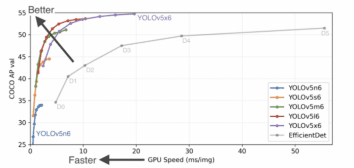
In October 2021, YOLOv5-v6.0 was released incorporating many new features and bug fixes (465 PRs from 73 contributors), bringing architecture tweaks, and the highlight introducing new P5 and P6 Nano models: YOLOv5n and YOLOv5n6. Nano models have ~75% fewer parameters, from 7.5M to 1.9M, than previous models, small enough to be run on mobile and CPU (shown in Figure 14). From the below figure, it is also evident that YOLOv5 outperforms the EfficientDet variants by significant margins. Furthermore, even the smallest YOLOv5 variant (i.e., YOLOv5n6) achieves comparable accuracy much faster than EfficientDet.

---

YOLOv5n Compared with YOLOv4-Tiny

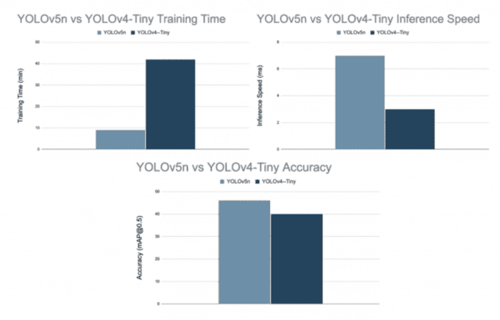
Since YOLOv5n is the smallest variant of YOLOv5, we compare it with YOLOv4-Tiny, which is also the lightest variant of the YOLOv4 model. Figure 15 shows that the YOLOv5 nano variant is hands-down better than YOLOv4-Tiny in terms of training time and accuracy.

---

PP-YOLO

Till now, we have seen YOLO in two different frameworks, namely Darknet and PyTorch; however, there is a third framework in which YOLO was implemented called PaddlePaddle framework, hence the name PP-YOLO. PaddlePaddle is a deep learning framework written by Baidu, which has a massive repository of Computer Vision and Natural Language Processing models.

Hardly four months into the release of YOLOv4, in Aug 2020, researchers of Baidu (Long et al.) published PP-YOLO: An Effective and Efficient Implementation of Object Detector. Similar to YOLOv4, the PP-YOLO object detector is also built based on YOLOv3 architecture.

---

PaddleDetection

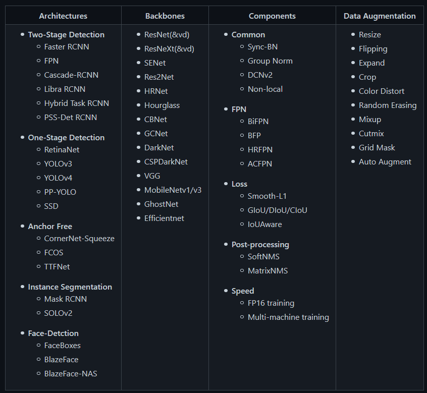
PP-YOLO is part of PaddleDetection, an end-to-end object detection development kit (shown in Figure 16) based on the PaddlePaddle framework. It provides a ton of object detection architectures, backbones, data augmentation techniques, components (like losses, feature pyramid network, etc.) that can be combined in different configurations to design the best object detection network.

In short, it provides image processing capabilities such as object detection, instance segmentation, multi-object tracking, keypoint detection, which ease the process of object detection in construction, training, optimization, and deployment of these models in a faster and better way.

Now let’s come back to the PP-YOLO paper.

The goal of the PP-YOLO paper was not to publish a novel object detection model but an object detector with relatively balanced effectiveness and efficiency that can be directly applied in actual application scenarios. And this goal resonates with the PaddleDetection development kit motivation. Hence, the novelty is to prove that the ensemble of these tricks and techniques better balances effectiveness and efficiency and provides an ablation study of how much each step helps the detector.

Similar to YOLOv4, this paper also tries to combine various existing tricks that do not increase the number of model parameters and FLOPs but improve the detector’s accuracy as much as possible and ensure the detector’s speed is almost unchanged. However, unlike YOLOv4, this paper did not explore different backbone networks (Darknet-53, ResNext50) and data augmentation methods, nor do they use Neural Architecture Search (NAS) to search for model hyperparameters.

---

PP-YOLO Performance

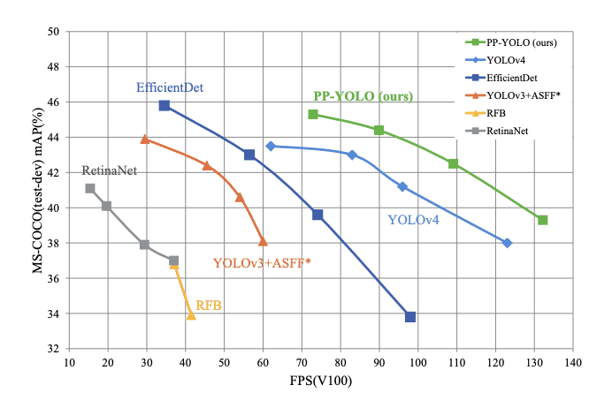
And by combining all of the tricks and techniques, when tested on a Volta 100 GPU with batch size = 1, PP-YOLO achieves 45.2% mAP and inference speed of 72.9 FPS (shown in Figure 17), signifying a better balance between effectiveness and efficiency, surpassing the famous state-of-the-art detectors such as EfficientDet, YOLOv4, and RetinaNet.

---

PP-YOLO Architecture

Single-Stage detection models are generally composed of backbone, detection neck, and detection head. The architecture of PP-YOLO (shown in Figure 18) is quite similar to YOLOv3 and YOLO4 detection models.

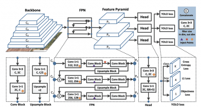
The PP-YOLO detector is divided into three parts:

• Backbone: The backbone in an object detector is a fully convolutional network that helps extract feature maps from the image. It is similar in spirit to a pre-trained image classification model. Instead of using the Darknet-53 architecture (in YOLOv3 and YOLOv4), the proposed model used a ResNet50-vd-dcn as the backbone.
  
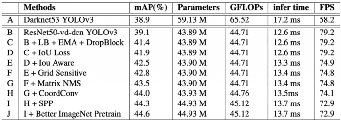
  In the proposed backbone model, the 3×3 convolution layer is replaced by deformable convolutions in the last stage of the architecture. The number of parameters and FLOPs of ResNet50-vd are much smaller than those of Darknet-53. This helped in achieving a slightly higher mAP of 39.1 compared to YOLOv3.

• Detection Neck: The Feature Pyramid Network (FPN) creates a pyramid of features by lateral connections between the feature maps. If you look closely at the below figure, feature maps from stages C3, C4, and C5 are fed as an input to the FPN module.

• Detection Head: The detection head is the final part of the object detection pipeline that predicts the bounding box (localization) and classification of the objects. The head of PP-YOLO is the same as the YOLOv3 head. Predicting the final output uses a 3×3 convolution layer followed by a 1×1 convolution layer.
  
  The output channels of the final output are , where is the number of classes (80 for MS COCO dataset), 3 is the number of anchors at each grid. For each anchor, the first K channels are the prediction class probabilities, four channels are the bounding box coordinates prediction, and one channel is the prediction of the objectness score.

In the above PP-YOLO architecture, the diamond inject points denote the coord-conv layers, purple triangles represent the DropBlocks, and the red star mark indicates the Spatial Pyramid Pooling.

---

Selection of Tricks and Techniques

If you remember, we discussed that this paper combines various tricks and techniques to design an effective and efficient object detection network; now, we will briefly go through each of them. These tricks are all already existing, coming from different papers.

• Larger Batch Size: Leveraging a larger batch size helps stabilize the training and lets the model produce better results. The batch size is changed from 64 to 192, and accordingly, the learning rate and training schedule are also updated.
• Exponential Moving Average: The authors claim that using moving averages of the trained parameters produced better results during inference.
• DropBlock Regularization: It is a technique similar to the Dropout regularization used to prevent overfitting. However, in Dropout block regularization, the dropped feature points are no longer spread randomly but are combined into blocks, and the entire block is dropped. So it is a structured dropout in which neurons from contiguous regions of a feature map are dropped together, as shown in Figure 19.

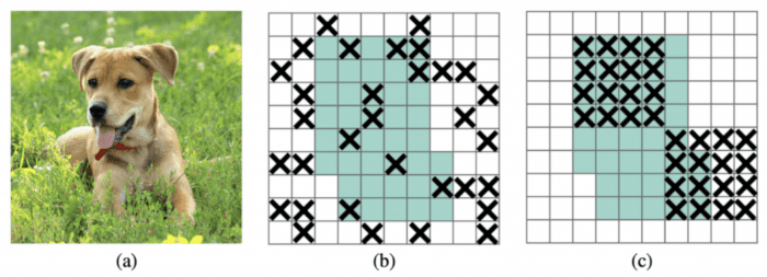
In PP-YOLO, DropBlock is only applied in the detection head (i.e., FPN) since adding it to the backbone tends to decrease the model’s performance.

• Intersection over Union (IoU) Loss: An extra loss (i.e., IoU loss) is added to train the model, while the existing L1 loss is used in YOLOv3, and most YOLO architectures are not replaced. An extra branch is added to calculate the IoU loss. This is done as the mAP evaluation metric strongly relies on the IoU.
• IoU Aware: Since localization accuracy is not considered in the final detection confidence, an IoU prediction branch is added to measure the localization accuracy. While during the inference predicted IoU score is multiplied by the classification probability and objectiveness score to predict the final detection confidence.
• Matrix Non-Maximum Suppression (NMS): A parallel implementation of a soft NMS version is used faster than traditional NMS and does not bring any loss of efficiency. The soft NMS works sequentially and cannot be implemented in parallel.
• Spatial Pyramid Pooling (SPP) Layer: The SPP layer implemented in YOLOv4 is applied in PP-YOLO as well but only in the top feature map. Adding SPP adds 2% of the model parameters and 1% FLOPS, but this lets the model increase the receptive field of the feature.
• Better Pretrained Model: A pre-trained model with better classification accuracy on ImageNet is used, resulting in better detection performance. A distilled ResNet50-vd model is used as the pretrain model.

---

Results

Earlier in the introduction of PP-YOLO, we learned that PP-YOLO runs faster than YOLOv4, with a better mean average precision score from 43.5% to 45.2%. The detailed performance of PP-YOLO is shown in Table 3.

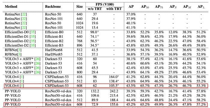
Long et al. (2020) compared the model on the Volta 100 GPU with and without TensorRT (to speed up inference).From the table, we can conclude that compared to YOLOv4, the mAP score on the MS COCO dataset increases from 43.5% to 45.2% and FPS from 62 to 72.9 (without TensorRT).

The table also shows PP-YOLO with other image resolutions, and it does seem that PP-YOLO has an advantage in the balance of speed and accuracy compared to other state-of-the-art detectors.

---

Ablation Study

The ablation study conducted by the authors shows how the tricks and techniques affect the parameter and performance of the model. In Table 4, the PP-YOLO starts from the second row denoted as B, where the detector uses ResNet50 as the backbone with deformable convolutions. As you move to the next row C, tricks are added to the previous model architecture, and throughout the same is followed. The performance gains and increase of parameters and FLOPS are shown in the corresponding columns.

We would highly recommend you to check out the paper for more details.

---

Scaled-YOLOv4

Wang et al. (2021) published a paper titled “Scaled-YOLOv4: Scaling Cross Stage Partial Network” at the CVPR conference. This paper has gathered more than 190 citations so far! With Scaled-YOLOv4, the authors have pushed the YOLOv4 model forward by efficiently scaling the network’s design and scale, surpassing the previous state-of-the-art EfficientDet published earlier this year by the Google Research Brain team.

The implementation of Scaled-YOLOv4 in the PyTorch framework can be found here.

The proposed detection network based on the Cross-Stage Partial approach scales both up and down, beating previous benchmarks from previous small and large object detection models on both ends of the speed and accuracy. In addition, the network scaling approach modifies the depth, width, resolution, and structure of the network.

Figure 20 shows the Scaled-YOLOv4-large model achieves state-of-the-art results: 55.5% AP (73.4% AP50) for the MS COCO dataset at a speed of ∼16 FPS on the Tesla V100 GPU.

On the other hand, the lighter version called Scaled-YOLOv4-tiny achieves 22.0% AP (42.0% AP50) at a speed of ∼443 FPS on RTX 2080Ti GPU while using TensorRT (with half-precision FP-16) optimization (batch size = 4).

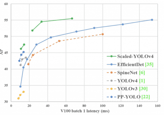
Figure 20 shows that Scaled-YOLOv4 achieves the best results compared to other state-of-the-art detectors.

---

What Is Model Scaling?

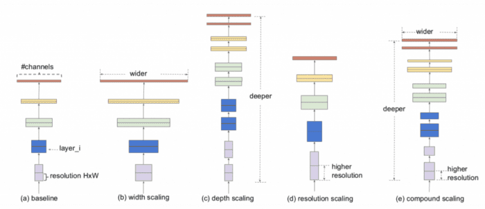
Convolutional neural network architecture can be scaled in three dimensions: depth, width, and resolution. The depth of the network corresponds to the number of layers in a network. The width is associated with the number of filters or channels in a convolutional layer. Finally, the resolution is simply the height and width of the input image.

Figure 21 gives a more intuitive understanding of model scaling across these three dimensions where (a) is a baseline network example; (b)-(d) are conventional scaling that only increases one dimension of network width, depth, or resolution; and (e) is a proposed (in EfficientDet) compound scaling method that uniformly scales all three dimensions with a fixed ratio.

The traditional model scaling method is to change the depth of a model, that is, to add more convolutional layers. For example, the VGGNet designed by Simonyan et al. stacked additional convolutional layers in different stages and used this concept to design VGG-16 and VGG-19 architectures.

The following methods generally follow the same methodology for model scaling. First, ResNet architecture proposed by He et al. (2015) used depth scaling to construct very deep networks, such as ResNet-50, ResNet-101, which allowed the network to learn more complex features but suffered from vanishing gradient problems. Later, Zagoruyko and Komodakis (2017) thought about the width of the network, and they changed the number of kernels of the convolutional layer to realize scaling, hence, wide ResNet (WRN), while maintaining the same accuracy. Although WRN had more parameters than ResNet, the inference speed was much faster.

Then in recent years, compound scaling uniformly scales all dimensions of depth/width/resolution of a convolutional neural network architecture using a compound coefficient. Unlike conventional practice that arbitrarily scales these factors, the compound scaling method uniformly scales network width, depth, and resolution with a set of fixed scaling coefficients.

And that’s what scaled-YOLOv4 also tries to do, that is, uses optimal network scaling techniques to achieve YOLOv4-CSP -> P5 -> P6 -> P7 detection networks.

---

Improvements in Scaled-YOLOv4 over YOLOv4

• Scaled-YOLOv4 uses optimal network scaling techniques to achieve YOLOv4-CSP -> P5 -> P6 -> P7 networks.
• Modified activations for width and height, which allows faster network training.
• Improved network architecture: Backbone optimized and Neck (Path-Aggregation Network) uses CSP connections and Mish activation.
• Exponential Moving Average (EMA) is used during the training.
• For each resolution of the network, a separate network is trained, while in YOLOv4 single network was trained on multiple resolutions.

---

Scaled-YOLOv4 Design

---

CSP-ized YOLOv4

YOLOv4 was designed for real-time object detection on a general GPU. In Scaled-YOLOv4, the YOLOv4 is re-designed to YOLOv4-CSP to get the best speed/accuracy trade-off.

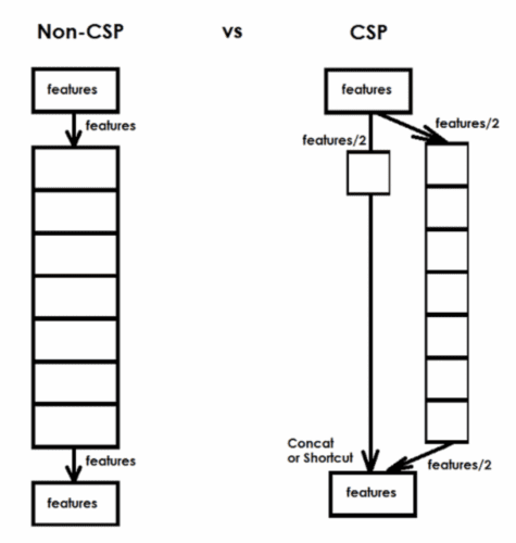
Wang et al. (2021) often mentioned in the paper that they “CSP-ized” a given portion of the object detection network. To CSP-ize here means to apply the concepts laid out in the Cross Stage Partial Networks paper. The CSP is a new way to architect convolutional neural networks that reduces computation for various CNN networks: up to 50% (for the Darknet backbone in FLOPs).

In a CSP connection:

• Half of the output signal goes along the main path that helps generate more semantic information with a large receptive field.
• The other half of the signal pivots help retain more spatial information with a small receptive field.

Figure 22 shows an example of a CSP connection. On the left is a standard network, while on the right is the CSP network.

---

Scaling the YOLOv4-Tiny Model

The YOLOv4-tiny model had different considerations than the Scaled-YOLOv4 model because, on edge, various constraints come into play, like memory bandwidth and memory access. For the YOLOv4-tiny’s shallow CNN, the authors look to OSANet for its favorable computational complexity at little depth.

Table 5 shows the performance comparison of YOLOv4-tiny with other tiny object detectors. Again, YOLOv4-tiny achieves the best performance in comparison with other tiny models.

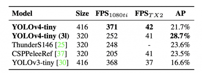
Table 6 shows the results of YOLOv4-tiny when tested on different embedded GPUs, including Xavier AGX, Xavier NX, Jetson TX2, Jetson NANO. If FP16 and batch size = 4 are adopted to test Xavier AGX and Xavier NX, the frame rate can reach 290 FPS and 118 FPS, respectively.

In addition, if one uses TensorRT FP16 to run YOLOv4-tiny on general GPU RTX 2080ti when the batch size, respectively, equals 1 and 4, the respective frame rate can reach 773 FPS and 1774 FPS, which is extremely fast.

YOLOv4-tiny can achieve real-time performance no matter which device is used.

---

Scaling the YOLOv4-CSP Models

To detect large objects in large images, the authors find that increasing the depth and number of stages in the CNN backbone and neck is essential (Increasing the width reportedly has little effect). This allows them first to scale up input size and number of stages and dynamically adjust width and depth according to real-time inference speed requirements. In addition to these scaling factors, authors also alter the configuration of their model’s architecture in the paper.

YOLOv4-large is designed for cloud GPU; the primary purpose is to achieve high accuracy for object detection. In addition, a fully CSP-ized model, YOLOv4-P5, is developed and scaled up to YOLOv4-P6 and YOLOv4-P7, as shown in Figure 23.

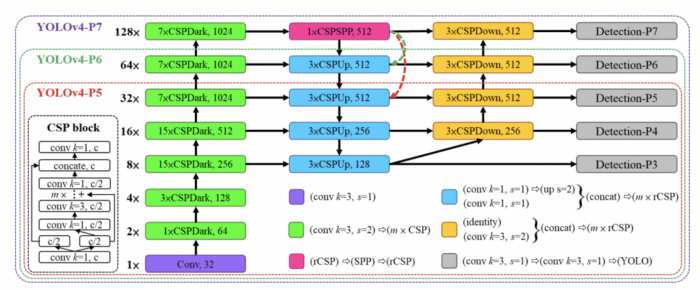
YOLOv4-P6 can reach real-time performance at 30 FPS on videos when the width scaling factor equals 1. YOLOv4-P7 can achieve real-time performance at 16 FPS on videos when the width scaling factor equals 1.25.

---

Data Augmentations

Data augmentation in YOLOv4 was one of the key contributions to YOLOv4’s impressive performance. In Scaled-YOLOv4, the authors first train on a less augmented dataset, then turn up the augmentations for fine-tuning at the end of training. They also use “Test Time Augmentations,” where several augmentations are applied to the test set. Predictions are then averaged across those test augmentations to boost their non-real-time results further.

To conclude, the authors show that the YOLOv4 object detection neural network based on the CSP approach scales both up and down and applies to small and large networks; hence, they call it Scaled-YOLOv4. Furthermore, the proposed model (YOLOv4-large) achieved the highest accuracy of 56.0% AP on the test-dev MS COCO dataset, extremely high speed 1774 FPS for the small model YOLOv4-tiny RTX 2080Ti by using TensorRT-FP16, and optimal speed and accuracy for other YOLOv4 models.

So far, we have covered seven YOLO object detectors, and we can say that for Object Detection, the Year 2020 was the best year by far and even more so for the YOLO family. We learned that one after the other state-of-the-art in object detection was reached by YOLOv4, YOLOv5, PP-YOLO, and Scaled-YOLOv4.

Let’s now move on to the next YOLO detector and see what was in store for the Year 2021!

---

PP-YOLOv2

In 2021, Baidu released the second version of PP-YOLO called PP-YOLOv2: A Practical Object Detector by Xing Huang et al. published on arXiv achieving new heights in the object detection domain.

From the title of the paper, one could easily infer that the motivation behind this paper was to develop an object detector that achieves good accuracy and performs inference at a faster speed. Hence, a practical object detector. Moreover, since this paper is a follow-up of previous work (i.e., PP-YOLO), the authors wanted to develop a detector that had a perfect balance between effectiveness and efficiency, and to achieve that, a similar analogy of ensembling tricks and techniques was followed with focus on ablation study.

By combining multiple effective refinements, PP-YOLOv2 significantly improved the performance (i.e., from 45.9% mAP to 49.5% mAP on MS COCO2017 test set). Furthermore, in terms of speed, PP-YOLOv2 runs in 68.9FPS at 640×640 image resolution, as shown in Figure 24. In addition, PPYOLOv2 was introduced with two different backbone architectures: ResNet-50 and ResNet-101, unlike PPYOLOv1, which was released with only the ResNet-50 backbone.

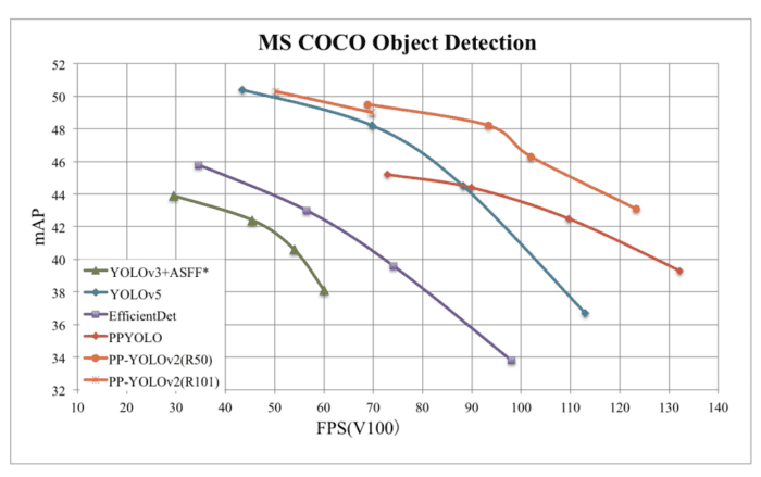
With the support of the TensorRT engine, on half-precision (FP16, batch size = 1) further improved PP-YOLOv2-ResNet50 inference speed to 106.5 FPS, surpassing the other state-of-the-art object detectors like YOLOv4-CSP and YOLOv5l with roughly the same amount of model parameters.

When the backbone of the detector was replaced from ResNet50 to ResNet101, PP-YOLOv2 achieved 50.3% mAP on the MS COCO2017 test set, achieving similar performance with YOLOv5x beating YOLOv5x significantly in the speed by almost 16%.

So now you know if your boss asks you to work on a problem that involves object detection, which detector you need to pick. Of course, the answer would be PP-YOLOv2 if the KPI is to achieve good performance at a much faster speed :)!

---

Revisiting PP-YOLO

By now, we know that PP-YOLOv2 builds on the research advancements made in the PP-YOLO paper, which acts as a baseline model for PP-YOLOv2.

PP-YOLO was an enhanced version of YOLOv3 in which the backbone was replaced with ResNet50-vd from Darknet-53. Many other improvements were made through a rigorous ablation study by leveraging a total of 10 tricks, such as

• DropBlock regularization
• Deformable Convolutions
• CoordConv
• Spatial Pyramid Pooling
• IoU loss and branch
• Grid Sensitivity
• Matrix NMS
• Better ImageNet pretraining model

---

Selection of Refinements

• Path Aggregation Network (PAN): To detect objects at different scales, the authors employ PAN in the neck of the object detection network. In PP-YOLO, Feature Pyramid Network was leveraged to compose bottom-up paths. Similar to YOLOv4, in PP-YOLOv2, the authors follow the design of PAN to aggregate the top-down information.
• Mish Activation Function: The mish activation function is adopted in the neck of the detection network; since PP-YOLOv2 used the pre-trained parameters because of its robust 82.4% top-1 accuracy on the ImageNet classification dataset. It was proved effective in the backbone of various practical object detectors like YOLOv4 and YOLOv5.
• Larger Input Size: Detecting smaller objects is often a challenge, and as the image traverses through the network, the information of the objects on a small scale is lost. Thus, in PP-YOLOv2, the input size is increased, enlarging the area of objects. As a result, performance will be increased. The largest input size, 608, is increased to 768. Since, larger input resolution occupies more memory, thus, the batch size is reduced from 24 images per GPU to 12 images per GPU drawing uniformly across different input sizes [320, 352, 384, 416, 448, 480, 512, 544, 576, 608, 640, 672, 704, 736, 768].
• IoU Aware Branch: In PP-YOLO, IoU aware loss is calculated in a soft weight format inconsistent with the original intention. Thus in PP-YOLOv2, a soft label format better tunes the PP-YOLO’s loss function and makes it more aware of the overlap between bounding boxes.

Table 7 shows the ablation study of refinements on the MS COCO mini validation split inference on the Volta 100 GPU. In the table, A refers to the baseline PP-YOLO model. Then, in B, PAN and Mish are added to A, giving a significant boost of 2 mAP; though B is slower than A, the accuracy jump is worth it.

YOLOv4 and YOLOv5 were evaluated on 640 image resolution, PP-YOLOv2’s input size is increased to 640 for training and evaluation to have a fair comparison (shown in C).

Incremental mAP gains in both D (larger input size) and E (IoU Aware Branch) are seen with no reduction in inference time, which is a good sign.

For more detailed information regarding the speed and accuracy comparison of PP-YOLOv2 with other state-of-the-art object detectors, check Table 2 in their paper on arXiv.

---

YOLOX

In 2021, Ge et al. published a technical report called YOLOX: Exceeding YOLO Series in 2021 on arXiv. Till now, the only anchor-free YOLO object detector we learned was YOLOv1, but YOLOX too detects objects in an anchor-free manner. Moreover, it also conducts other advanced detection techniques like decoupled head, leverage robust data augmentation techniques, and leading label assignment strategy SimOTA to achieve state-of-the-art results.

YOLOX won the 1st Place on Streaming Perception Challenge (Workshop on Autonomous Driving conducted in conjunction with CVPR 2021) using a single YOLOX-L model.

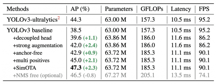
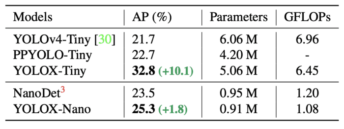
As shown in Figure 25 (right), YOLOX-Nano, with only 0.91M parameters, achieved 25.3% AP on the MS COCO dataset, surpassing NanoDet by 1.8% AP. Adding various modifications to YOLOv3 boosted the accuracy from 44.3% to 47.3% AP on COCO.

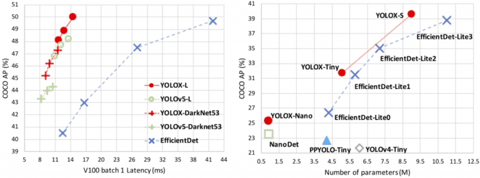
YOLOX-L achieved 50.0% AP on COCO at a speed of 68.9 FPS on Tesla V100 with roughly the same parameters as YOLOv4- CSP, YOLOv5-L, exceeding YOLOv5-L by 1.8% AP.

YOLOX was implemented in the PyTorch framework and was designed keeping in mind the practical use by the developers and researchers. Therefore, the YOLOX deploy versions have also been made available in ONNX, TensorRT, and OpenVino frameworks.

Over the past 2 years, significant advances in object detection academia have focused on anchor-free detectors, advanced label assignment strategies, and end-to-end (NMS-free) detectors. However, none of these techniques have been applied to YOLO object detection architectures yet, including the recent models: YOLOv4, YOLOv5, and PP-YOLO. Most of them are still anchor-based detectors with handcrafted assigning rules for training. And that’s the motivation behind publishing YOLOX!

---

YOLOX-Darknet53

YOLOv3 with Darknet-53 backbone is selected as the baseline. Then, a series of improvements were made to the base model.

The training settings are primarily similar from the baseline to the final YOLOX model. All the models were trained for 300 epochs on the MS COCO train2017 dataset with a batch size of 128. The input size is evenly drawn from 448 to 832 with 32 strides. FPS and latency were measured with FP16-precision (half-precision) and batch size = 1 on a single Tesla Volta 100 GPU.

---

YOLOv3-Baseline

It uses the DarkNet-53 backbone and an SPP layer referred to as YOLOv3-SPP. Some training strategies are modified compared to the original implementation, such as

• Exponential Moving Average weights update
• Cosine learning rate schedule
• BCE Loss for classification and objectness branch
• IoU Loss for regression branch

With those enhancements, the YOLOv3 baseline achieved 38.5% AP on the MS COCO validation set, as shown in Table 8. All models are tested at 640×640 resolution, with FP16-precision and batch size = 1 on a Tesla V100. The latency and FPS in the below table are measured without post-processing.

---

Decoupled Head

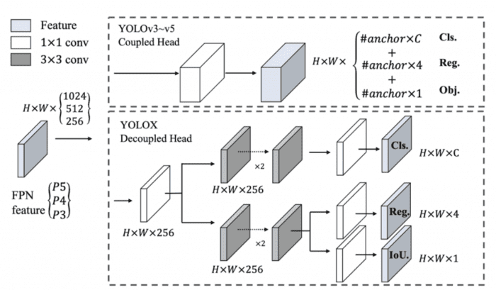
Figure 26 shows the coupled head (top) used in YOLOv3 to YOLOv5 models and decoupled head (bottom) in YOLOX. The head here means the output prediction at different scales. For example, in the coupled head, we have a prediction tensor (the detailed explanation is shown in the below figure). And the problem with this way is that usually, we have the classification and localization tasks in the same head during the training, which often compete with each other during the training. As a result, the model struggles to classify and localize each object in the image correctly.

Thus, the decoupled head for classification and localization is used in YOLOX, as shown in Figure 26 (bottom). For each level of the FPN feature, first, a 1×1 conv layer is applied to reduce the feature channels to 256. Then two parallel branches are added with two 3×3 conv layers, for classification and localization tasks, respectively. Finally, an extra IoU branch is added to the localization branch.

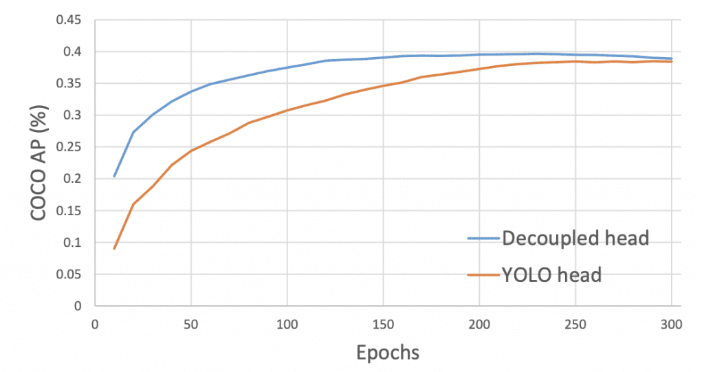
The decoupled head permits the YOLOX model to converge faster than the coupled head, as shown in Figure 27. Furthermore, on the x-axis, we can observe how the COCO AP scores improve much faster for the decoupled head than the YOLOv3 head.

---

Strong Data Augmentation

Mosaic and MixUp data augmentation techniques similar to YOLOv4 were added to boost YOLOX performance. Mosaic is an efficient augmentation strategy proposed by ultralytics-YOLOv3.

Using the above two augmentation techniques, the authors found that pre-training the backbone on the ImageNet dataset was no more beneficial, so they trained the model from scratch.

---

Anchor-Free Detection

To develop a high-speed object detector, the YOLOX adopted an anchor-free mechanism that reduces the number of design parameters since now we don’t have to deal with the anchor boxes anymore, which increased the number of predictions significantly. And so, for each location or grid in the prediction head, we now have only one prediction instead of predicting output for three different anchor boxes. Each object’s center location is considered a positive sample, and there is a predefined scaled range.

Simply put, in anchor-free detection, the predictions for each grid are reduced from 3 to 1, and it directly predicts four values, that is, two offsets in terms of the top-left corner of the grid and the height and width of the predicted box.

With this approach, the network parameters and GFLOPs of the detector are reduced, and it makes the detector faster and not just that even the performance improves to 42.9% AP, as shown in Table 8.

---

Multi-Positives

To be consistent with the assigning rule of YOLOv3, the anchor-free version selects only ONE positive sample (the center location) for each object while ignoring other high-quality predictions. However, optimizing those high-quality predictions may also bring beneficial gradients, which may alleviate the extreme imbalance of positive/negative sampling during training. In YOLOX, the center 3×3 area is assigned as positives, also named “center sampling” in the FCOS paper. As a result, the detector’s performance improves to 45.0% AP, as shown in Table 2.

---

Other Backbones

---

Modified CSPNet in YOLOv5

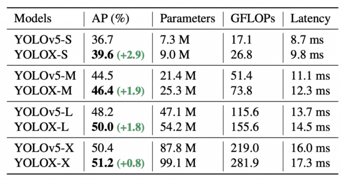
To have a fair comparison, YOLOX replaces the Darknet-53 backbone with YOLOv5’s modified CSP v5 backbone along with SiLU activation and the PAN head. By leveraging its scaling rule YOLOX-S, YOLOX-M, YOLOX-L, and YOLOX-X models are produced.

Table 9 shows a comparison between YOLOv5 models and YOLOX produced models. All the YOLOX variants show a consistent improvement by ∼3.0% to ∼1.0% AP, with only a marginal time increase coming from using the decoupled head. The models below were tested at 640×640 image resolution, with FP16-precision (half-precision) and batch size = 1 on a Tesla Volta 100 GPU.

---

Tiny and Nano Detectors

We compared YOLOX models with YOLOv5, which were small, medium, large, and extra-large in size (more parameters). The authors went one step further and shrunk the YOLOX models to have parameters lower than the YOLOX-S variant to produce YOLOX-Tiny and YOLOX-Nano. The YOLOX-Nano was designed especially for mobile devices. To construct this model, depth-wise convolution was adopted, resulting in a model with only 0.91M parameters and 1.08G FLOPs.

As shown in Table 10, YOLOX-Tiny is compared with YOLOv4-Tiny and PPYOLO-Tiny. Again, YOLOX performs well with an even smaller model size than its counterparts.

---

---

Summary

Congratulations on making it this far. If you were able to follow along easily or even with a little more effort, well done! So let’s quickly summarize:

1. We started the tutorial by introducing object detection: how object detection is different from image classification, challenges in detection, and what are single-stage and two-stage object detectors.
2. You were then introduced to the first single-stage detector called YOLOv1.
3. Then we briefly covered YOLOv2, YOLOv3, and YOLOv4.
4. Next, we discussed YOLOv5 developed by Ultralytics, the first YOLO model implemented in PyTorch after YOLOv4.
5. Then came PP-YOLO implemented in PaddlePaddle framework by Baidu, which showed promising results outperforming YOLOv4 and EfficientDet.
6. An extension of YOLOv4 called Scaled-YOLOv4 was then discussed, based on the Cross-Stage Partial approach scaling both up and down, beating previous benchmarks from previous small and large object detection models like EfficientDet, YOLOv4, and PP-YOLO in both speed and accuracy.
7. Then we discussed the second version of PP-YOLO, known as PP-YOLOv2, which made various refinements to PP-YOLO, thereby significantly improving the performance (i.e., from 45.9% mAP to 49.5% mAP) on the MS COCO2017 test set.
8. We then discussed YOLOX, an Anchor-Free object detection network after YOLOv1. YOLOX won the 1st Place on Streaming Perception Challenge in the CVPR workshop and outperformed the YOLOv5 large and nano models both in accuracy and speed.

---

References

1. https://alexeyab84.medium.com/scaled-yolo-v4-is-the-best-neural-network-for-object-detection-on-ms-coco-dataset-39dfa22fa982
2. https://blog.roboflow.com/scaled-yolov4-tops-efficientdet/

---

Citation Information

Sharma, A. “Introduction to the YOLO Family,” PyImageSearch, D. Chakraborty, P. Chugh, A. R. Gosthipaty, S. Huot, K. Kidriavsteva, R. Raha, and A. Thanki, eds., 2022, https://pyimg.co/dgbvi

@incollection{Sharma_2022_YOLO_Intro,
  author = {Aditya Sharma},
  title = {Introduction to the {YOLO} Family},
  booktitle = {PyImageSearch},
  editor = {Devjyoti Chakraborty and Puneet Chugh and Aritra Roy Gosthipaty and Susan Huot and Kseniia Kidriavsteva and Ritwik Raha and Abhishek Thanki},
  year = {2022},
  note = {https://pyimg.co/dgbvi},
}

---