OpenCV Super Resolution with Deep Learning

In this tutorial you will learn how to perform super resolution in images and real-time video streams using OpenCV and Deep Learning.

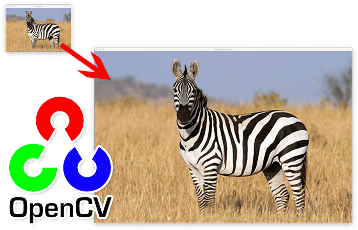
Today’s blog post is inspired by an email I received from PyImageSearch reader, Hisham:

“Hi Adrian, I read your Deep Learning for Computer Vision with Python book and went through your super resolution implementation with Keras and TensorFlow. It was super helpful, thank you.

I was wondering:

Are there any pre-trained super resolution models compatible with OpenCV’s dnn module?

Can they work in real-time?

If you have any suggestions, that would be a big help.”

You’re in luck, Hisham — there are super resolution deep neural networks that are both:

1. Pre-trained (meaning you don’t have to train them yourself on a dataset)
2. Compatible with OpenCV

However, OpenCV’s super resolution functionality is actually “hidden” in a submodule named in dnn_superres in an obscure function called DnnSuperResImpl_create.

The function requires a bit of explanation to use, so I decided to author a tutorial on it; that way everyone can learn how to use OpenCV’s super resolution functionality.

By the end of this tutorial, you’ll be able to perform super resolution with OpenCV in both images and real-time video streams!

To learn how to use OpenCV for deep learning-based super resolution, just keep reading.

OpenCV Super Resolution with Deep Learning

In the first part of this tutorial, we will discuss:

• What super resolution is
• Why we can’t use simple nearest neighbor, linear, or bicubic interpolation to substantially increase the resolution of images
• How specialized deep learning architectures can help us achieve super resolution in real-time

From there, I’ll show you how to implement OpenCV super resolution with both:

1. Images
2. Real-time video resolutions

We’ll wrap up this tutorial with a discussion of our results.

What is super resolution?

Super resolution encompases a set of algorithms and techniques used to enhance, increase, and upsample the resolution of an input image. More simply, take an input image and increase the width and height of the image with minimal (and ideally zero) degradation in quality.

That’s a lot easier said than done.

Anyone who has ever opened a small image in Photoshop or GIMP and then tried to resize it knows that the output image ends up looking pixelated.

That’s because Photoshop, GIMP, Image Magick, OpenCV (via the cv2.resize function), etc. all use classic interpolation techniques and algorithms (ex., nearest neighbor interpolation, linear interpolation, bicubic interpolation) to increase the image resolution.

These functions “work” in the sense that an input image is presented, the image is resized, and then the resized image is returned to the calling function …

… however, if you increase the spatial dimensions too much, then the output image appears pixelated, has artifacts, and in general, just looks “aesthetically unpleasing” to the human eye.

For example, let’s consider the following figure:

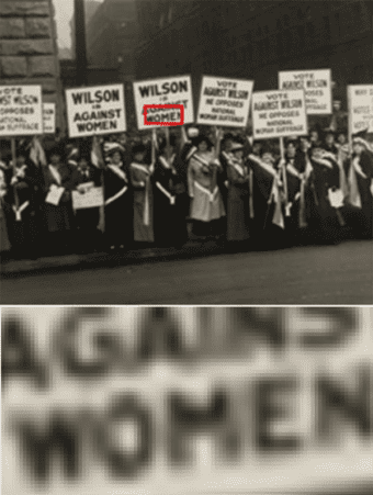
On the top we have our original image. The area highlighted in the red rectangle is the area we wish to extract and increase the resolution of (i.e., resize to a larger width and height without degrading the quality of the image patch).

On the bottom we have the output of applying bicubic interpolation, the standard interpolation method used for increasing the size of input images (and what we commonly use in cv2.resize when needing to increase the spatial dimensions of an input image).

However, take a second to note how pixelated, blurry, and just unreadable the image patch is after applying bicubic interpolation.

That raises the question:

Is there a better way to increase the resolution of the image without degrading the quality?

The answer is yes — and it’s not magic either. By applying novel deep learning architectures, we’re able to generate high resolution images without these artifacts:

Again, on the top we have our original input image. In the middle we have low quality resizing after applying bicubic interpolation. And on the bottom we have the output of applying our super resolution deep learning model.

The difference is like night and day. The output deep neural network super resolution model is crisp, easy to read, and shows minimal signs of resizing artifacts.

In the rest of this tutorial, I’ll uncover this “magic” and show you how to perform super resolution with OpenCV!

OpenCV super resolution models

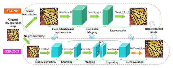
We’ll be utilizing four pre-trained super resolution models in this tutorial. A review of the model architectures, how they work, and the training process of each respective model is outside the scope of this guide (as we’re focusing on implementation only).

If you would like to read more about these models, I’ve included their names, implementations, and paper links below:

• EDSR: Enhanced Deep Residual Networks for Single Image Super-Resolution (implementation)
• ESPCN: Real-Time Single Image and Video Super-Resolution Using an Efficient Sub-Pixel Convolutional Neural Network (implementation)
• FSRCNN: Accelerating the Super-Resolution Convolutional Neural Network (implementation)
• LapSRN: Fast and Accurate Image Super-Resolution with Deep Laplacian Pyramid Networks (implementation)

A big thank you to Taha Anwar from BleedAI for putting together his guide on OpenCV super resolution, which curated much of this information — it was immensely helpful when authoring this piece.

Configuring your development environment for super resolution with OpenCV

In order to apply OpenCV super resolution, you must have OpenCV 4.3 (or greater) installed on your system. While the dnn_superes module was implemented in C++ back in OpenCV 4.1.2, the Python bindings were not implemented until OpenCV 4.3.

Luckily, OpenCV 4.3+ is pip-installable:

$ pip install opencv-contrib-python

If you need help configuring your development environment for OpenCV 4.3+, I highly recommend that you read my pip install OpenCV guide — it will have you up and running in a matter of minutes.

Having problems configuring your development environment?

All that said, are you:

• Short on time?
• Learning on your employer’s administratively locked system?
• Wanting to skip the hassle of fighting with the command line, package managers, and virtual environments?
• Ready to run the code right now on your Windows, macOS, or Linux system?

Then join PyImageSearch Plus today!

Gain access to Jupyter Notebooks for this tutorial and other PyImageSearch guides that are pre-configured to run on Google Colab’s ecosystem right in your web browser! No installation required.

And best of all, these Jupyter Notebooks will run on Windows, macOS, and Linux!

Project structure

With our development environment configured, let’s move on to reviewing our project directory structure:

$ tree . --dirsfirst
.
├── examples
│   ├── adrian.png
│   ├── butterfly.png
│   ├── jurassic_park.png
│   └── zebra.png
├── models
│   ├── EDSR_x4.pb
│   ├── ESPCN_x4.pb
│   ├── FSRCNN_x3.pb
│   └── LapSRN_x8.pb
├── super_res_image.py
└── super_res_video.py

2 directories, 10 files

Here you can see that we have two Python scripts to review today:

1. super_res_image.py: Performs OpenCV super resolution in images loaded from disk
2. super_res_video.py: Applies super resolution with OpenCV to real-time video streams

We’ll be covering the implementation of both Python scripts in detail later in this post.

From there, we have four super resolution models:

1. EDSR_x4.pb: Model from the Enhanced Deep Residual Networks for Single Image Super-Resolution paper — increases the input image resolution by 4x
2. ESPCN_x4.pb: Super resolution model from Real-Time Single Image and Video Super-Resolution Using an Efficient Sub-Pixel Convolutional Neural Network — increases resolution by 4x
3. FSRCNN_x3.pb: Model from Accelerating the Super-Resolution Convolutional Neural Network — increases image resolution by 3x
4. LapSRN_x8.pb: Super resolution model from Fast and Accurate Image Super-Resolution with Deep Laplacian Pyramid Networks — increases image resolution by 8x

Finally, the examples directory contains example input images that we’ll be applying OpenCV super resolution to.

Implementing OpenCV super resolution with images

We are now ready to implement OpenCV super resolution in images!

Open up the super_res_image.py file in your project directory structure, and let’s get to work:

# import the necessary packages
import argparse
import time
import cv2
import os

# construct the argument parser and parse the arguments
ap = argparse.ArgumentParser()
ap.add_argument("-m", "--model", required=True,
	help="path to super resolution model")
ap.add_argument("-i", "--image", required=True,
	help="path to input image we want to increase resolution of")
args = vars(ap.parse_args())

From there, Lines 8-13 parse our command line arguments. We only need two command line arguments here:

1. --model: The path to the input OpenCV super resolution model
2. --image: The path to the input image that we want to apply super resolution to

Given our super resolution model path, we now need to extract the model name and the model scale (i.e., factor by which we’ll be increasing the image resolution):

# extract the model name and model scale from the file path
modelName = args["model"].split(os.path.sep)[-1].split("_")[0].lower()
modelScale = args["model"].split("_x")[-1]
modelScale = int(modelScale[:modelScale.find(".")])

Line 16 extracts the modelName, which can be EDSR, ESPCN, FSRCNN, or LapSRN, respectively. The modelNamehas to be one of these model names; otherwise, the dnn_superres module and DnnSuperResImpl_create function will not work.

With the model name and scale parsed, we can now move on to loading the OpenCV super resolution model:

# initialize OpenCV's super resolution DNN object, load the super
# resolution model from disk, and set the model name and scale
print("[INFO] loading super resolution model: {}".format(
	args["model"]))
print("[INFO] model name: {}".format(modelName))
print("[INFO] model scale: {}".format(modelScale))
sr = cv2.dnn_superres.DnnSuperResImpl_create()
sr.readModel(args["model"])
sr.setModel(modelName, modelScale)

We start by instantiating an instance of DnnSuperResImpl_create, which is our actual super resolution object.

A call to readModel loads our OpenCV super resolution model from disk.

We then have to make a call to setModel to explicitly set the modelName and modelScale.

Failing to either read the model from disk or set the model name and scale will result in our super resolution script either erroring out or segfaulting.

Let’s now perform super resolution with OpenCV:

# load the input image from disk and display its spatial dimensions
image = cv2.imread(args["image"])
print("[INFO] w: {}, h: {}".format(image.shape[1], image.shape[0]))

# use the super resolution model to upscale the image, timing how
# long it takes
start = time.time()
upscaled = sr.upsample(image)
end = time.time()
print("[INFO] super resolution took {:.6f} seconds".format(
	end - start))

# show the spatial dimensions of the super resolution image
print("[INFO] w: {}, h: {}".format(upscaled.shape[1],
	upscaled.shape[0]))

Lines 31 and 32 load our input --image from disk and display the original width and height.

From there, Line 37 makes a call to sr.upsample, supplying the original input image. The upsample function, as the name suggests, performs a forward pass of our OpenCV super resolution model, returning the upscaled image.

We take care to measure the wall time for how long the super resolution process takes, followed by displaying the new width and height of our upscaled image to our terminal.

For comparison, let’s apply standard bicubic interpolation and time how long it takes:

# resize the image using standard bicubic interpolation
start = time.time()
bicubic = cv2.resize(image, (upscaled.shape[1], upscaled.shape[0]),
	interpolation=cv2.INTER_CUBIC)
end = time.time()
print("[INFO] bicubic interpolation took {:.6f} seconds".format(
	end - start))

Bicubic interpolation is the standard algorithm used to increase the resolution of an image. This method is implemented in nearly every image processing tool and library, including Photoshop, GIMP, Image Magick, PIL/PIllow, OpenCV, Microsoft Word, Google Docs, etc. — if a piece of software needs to manipulate images, it more than likely implements bicubic interpolation.

Finally, let’s display the output results to our screen:

# show the original input image, bicubic interpolation image, and
# super resolution deep learning output
cv2.imshow("Original", image)
cv2.imshow("Bicubic", bicubic)
cv2.imshow("Super Resolution", upscaled)
cv2.waitKey(0)

Here we display our original input image, the bicubic resized image, and finally our upscaled super resolution image.

We display the three results to our screen so we can easily compare results.

OpenCV super resolution results

Start by making sure you’ve used the “Downloads” section of this tutorial to download the source code, example images, and pre-trained super resolution models.

From there, open up a terminal, and execute the following command:

$ python super_res_image.py --model models/EDSR_x4.pb --image examples/adrian.png
[INFO] loading super resolution model: models/EDSR_x4.pb
[INFO] model name: edsr
[INFO] model scale: 4
[INFO] w: 100, h: 100
[INFO] super resolution took 1.183802 seconds
[INFO] w: 400, h: 400
[INFO] bicubic interpolation took 0.000565 seconds

In the top we have our original input image. In the middle we have applied the standard bicubic interpolation image to increase the dimensions of the image. Finally, the bottom shows the output of the EDSR super resolution model (increasing the image dimensions by 4x).

If you study the two images, you’ll see that the super resolution images appear “more smooth.” In particular, take a look at my forehead region. In the bicubic image, there is a lot of pixelation going on — but in the super resolution image, my forehead is significantly more smooth and less pixelated.

The downside to the EDSR super resolution model is that it’s a bit slow. Standard bicubic interpolation could take a 100x100px image and increase it to 400x400px at the rate of > 1700 frames per second.

EDSR, on the other hand, takes greater than one second to perform the same upsampling. Therefore, EDSR is not suitable for real-time super resolution (at least not without a GPU).

Note: All timings here were collected with a 3 GHz Intel Xeon W processor. A GPU was not used.

Let’s try another image, this one of a butterfly:

$ python super_res_image.py --model models/ESPCN_x4.pb --image examples/butterfly.png
[INFO] loading super resolution model: models/ESPCN_x4.pb
[INFO] model name: espcn
[INFO] model scale: 4
[INFO] w: 400, h: 240
[INFO] super resolution took 0.073628 seconds
[INFO] w: 1600, h: 960
[INFO] bicubic interpolation took 0.000833 seconds

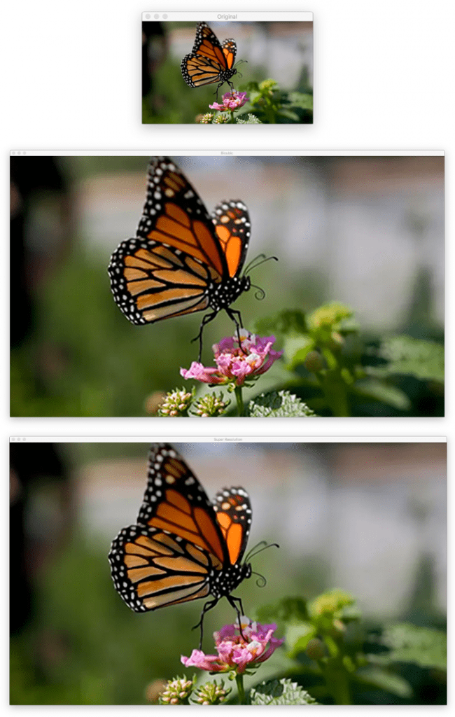
Again, on the top we have our original input image. After applying standard bicubic interpolation we have the middle image. And on the bottom we have the output of applying the ESPCN super resolution model.

The best way you can see the difference between these two super resolution models is to study the butterfly’s wings. Notice how the bicubic interpolation method looks more noisy and distorted, while the ESPCN output image is significantly more smooth.

The good news here is that the ESPCN model is significantly faster, capable of taking a 400x240px image and upsampling it to a 1600x960px model at the rate of 13 FPS on a CPU.

The next example applies the FSRCNN super resolution model:

$ python super_res_image.py --model models/FSRCNN_x3.pb --image examples/jurassic_park.png
[INFO] loading super resolution model: models/FSRCNN_x3.pb
[INFO] model name: fsrcnn
[INFO] model scale: 3
[INFO] w: 350, h: 197
[INFO] super resolution took 0.082049 seconds
[INFO] w: 1050, h: 591
[INFO] bicubic interpolation took 0.001485 seconds

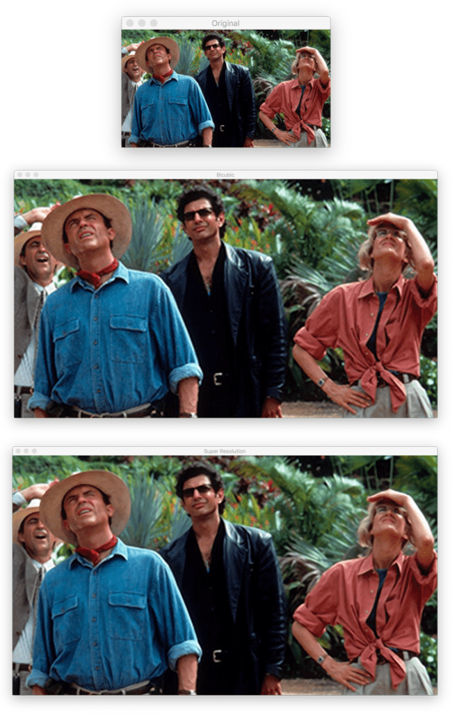
Pause a second and take a look at Allen Grant’s jacket (the man wearing the blue denim shirt). In the bicubic interpolation image, this shirt is grainy. But in the FSRCNN output, the jacket is far more smoothed.

Similar to the ESPCN super resolution model, FSRCNN took only 0.08 seconds to upsample the image (a rate of ~12 FPS).

Finally, let’s look at the LapSRN model, which will increase our input image resolution by 8x:

$ python super_res_image.py --model models/LapSRN_x8.pb --image examples/zebra.png
[INFO] loading super resolution model: models/LapSRN_x8.pb
[INFO] model name: lapsrn
[INFO] model scale: 8
[INFO] w: 400, h: 267
[INFO] super resolution took 4.759974 seconds
[INFO] w: 3200, h: 2136
[INFO] bicubic interpolation took 0.008516 seconds

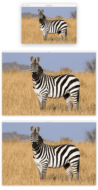
Perhaps unsurprisingly, this model is the slowest, taking over 4.5 seconds to increase the resolution of a 400x267px input to an output of 3200x2136px. Given that we are increasing the spatial resolution by 8x, this timing result makes sense.

That said, the output of the LapSRN super resolution model is fantastic. Look at the zebra stripes between the bicubic interpolation output (middle) and the LapSRN output (bottom). The stripes on the zebra are crisp and defined, unlike the bicubic output.

Implementing real-time super resolution with OpenCV

We’ve seen super resolution applied to single images — but what about real-time video streams?

Is it possible to perform OpenCV super resolution in real-time?

The answer is yes, it’s absolutely possible — and that’s exactly what our super_res_video.py script does.

Note: Much of the super_res_video.py script is similar to our super_res_image.py script, so I will spend less time explaining the real-time implementation. Refer back to the previous section on “Implementing OpenCV super resolution with images” if you need additional help understanding the code.

Let’s get started:

# import the necessary packages
from imutils.video import VideoStream
import argparse
import imutils
import time
import cv2
import os

# construct the argument parser and parse the arguments
ap = argparse.ArgumentParser()
ap.add_argument("-m", "--model", required=True,
	help="path to super resolution model")
args = vars(ap.parse_args())

Lines 2-7 import our required Python packages. These are all near-identical to our previous script on super resolution with images, with the exception of my imutils library and the VideoStream implementation from it.

We then parse our command line arguments. Only a single argument is required, --model, which is the path to our input super resolution model.

Next, let’s extract the model name and model scale, followed by loading our OpenCV super resolution model from disk:

# extract the model name and model scale from the file path
modelName = args["model"].split(os.path.sep)[-1].split("_")[0].lower()
modelScale = args["model"].split("_x")[-1]
modelScale = int(modelScale[:modelScale.find(".")])

# initialize OpenCV's super resolution DNN object, load the super
# resolution model from disk, and set the model name and scale
print("[INFO] loading super resolution model: {}".format(
	args["model"]))
print("[INFO] model name: {}".format(modelName))
print("[INFO] model scale: {}".format(modelScale))
sr = cv2.dnn_superres.DnnSuperResImpl_create()
sr.readModel(args["model"])
sr.setModel(modelName, modelScale)

# initialize the video stream and allow the camera sensor to warm up
print("[INFO] starting video stream...")
vs = VideoStream(src=0).start()
time.sleep(2.0)

Lines 16-18 extract our modelName and modelScale from the input --model file path.

Using that information, we instantiate our super resolution (sr) object, load the model from disk, and set the model name and scale (Lines 26-28).

We then initialize our VideoStream (such that we can read frames from our webcam) and allow the camera sensor to warm up.

With our initializations taken care of, we can now loop over frames from the VideoStream:

# loop over the frames from the video stream
while True:
	# grab the frame from the threaded video stream and resize it
	# to have a maximum width of 300 pixels
	frame = vs.read()
	frame = imutils.resize(frame, width=300)

	# upscale the frame using the super resolution model and then
	# bicubic interpolation (so we can visually compare the two)
	upscaled = sr.upsample(frame)
	bicubic = cv2.resize(frame,
		(upscaled.shape[1], upscaled.shape[0]),
		interpolation=cv2.INTER_CUBIC)

Line 36 starts looping over frames from our video stream. We then grab the next frame and resize it to have a width of 300px.

We perform this resizing operation for visualization/example purposes. Recall that the point of this tutorial is to apply super resolution with OpenCV. Therefore, our example should show how to take a low resolution input and then generate a high resolution output (which is exactly why we are reducing the resolution of the frame).

Line 44 resizes the input frame using our OpenCV resolution model, resulting in the upscaled image.

Lines 45-47 apply basic bicubic interpolation so we can compare the two methods.

Our final code block displays the results to our screen:

# show the original frame, bicubic interpolation frame, and super
	# resolution frame

	cv2.imshow("Original", frame)
	cv2.imshow("Bicubic", bicubic)
	cv2.imshow("Super Resolution", upscaled)
	key = cv2.waitKey(1) & 0xFF

	# if the `q` key was pressed, break from the loop
	if key == ord("q"):
		break

# do a bit of cleanup
cv2.destroyAllWindows()
vs.stop()

Here we display the original frame, bicubic interpolation output, as well as the upscaled output from our super resolution model.

We continue processing and displaying frames to our screen until a window opened by OpenCV is clicked and the q is pressed, causing our Python script to quit/exit.

Finally, we perform a bit of cleanup by closing all windows opened by OpenCV and stopping our video stream.

Real-time OpenCV super resolution results

Let’s now apply OpenCV super resolution in real-time video streams!

Make sure you’ve used the “Downloads” section of this tutorial to download the source code, example images, and pre-trained models.

From there, you can open up a terminal and execute the following command:

$ python super_res_video.py --model models/FSRCNN_x3.pb
[INFO] loading super resolution model: models/FSRCNN_x3.pb
[INFO] model name: fsrcnn
[INFO] model scale: 3
[INFO] starting video stream...

Here you can see that I’m able to run the FSRCNN model in real-time on my CPU (no GPU required!).

Furthermore, if you compare the result of bicubic interpolation with super resolution, you’ll see that the super resolution output is much cleaner.

Suggestions

It’s hard to show all the subtleties that super resolution gives us in a blog post with limited dimensions to show example images and video, so I strongly recommend that you download the code/models and study the outputs close-up.

Summary

In this tutorial you learned how to implement OpenCV super resolution in both images and real-time video streams.

Basic image resizing algorithms such as nearest neighbor interpolation, linear interpolation, and bicubic interpolation can only increase the resolution of an input image to a certain factor — afterward, image quality degrades to the point where images look pixelated, and in general, the resized image is just aesthetically unpleasing to the human eye.

Deep learning super resolution models are able to produce these higher resolution images while at the same time helping prevent much of these pixelations, artifacts, and unpleasing results.

That said, you need to set the expectation that there are no magical algorithms like you see in TV/movies that take a blurry, thumbnail-sized image and resize it to be a poster that you could print out and hang on your wall — that simply isn’t possible.

That said, OpenCV’s super resolution module can be used to apply super resolution. Whether or not that’s appropriate for your pipeline is something that should be tested:

1. Try first using cv2.resize and standard interpolation algorithms (and time how long the resizing takes).
2. Then, run the same operation, but instead swap in OpenCV’s super resolution module (and again, time how long the resizing takes).

Compare both the output and the amount of time it took both standard interpolation and OpenCV super resolution to run. From there, select the resizing mode that achieves the best balance between the quality of the output image along with the time it took for the resizing to take place.

To download the source code to this post (and be notified when future tutorials are published here on PyImageSearch), simply enter your email address in the form below!