There were three huge influences in my life that made me want to become a scientist.
The first was David A. Johnston, an American USGS volcanologist who died on May 18th, 1980, the day of the catastrophic eruption of Mount St. Helens in Washington state. He was the first to report the eruption, exclaiming “Vancouver! Vancouver! This is it!” moments before he died in the lateral blast of the volcano. I felt inspired by his words. He knew at that moment that he was going to die — but he was excited for the science, for what he had so tediously studied and predicted had become reality. He died studying what he loved. If we could all be so lucky.
The second inspiration was actually a melding of my childhood hobbies. I loved to build things out of plastic and cardboard blocks. I loved crafting structures out of nothing more than rolled up paper and Scotch tape — at first, I thought I wanted to be an architect.
But a few years later I found another hobby. Writing. I spent my time writing fictional short stories and selling them to my parents for a quarter. I guess I also found that entrepreneurial gene quite young. For a few years after, I felt sure that I was going to be an author when I grew up.
My final inspiration was Jurassic Park. Yes. Laugh if you want. But the dichotomy of scientists between Alan Grant and Ian Malcolm was incredibly inspiring to me at a young age. On one hand, you had the down-to-earth, get-your-hands-dirty demeanor of Alan Grant. And on the other you had the brilliant mathematician (err, excuse me, chaotician) rock star. They represented two breeds of scientists. And I felt sure that I was going to end up like one of them.
Fast forward through my childhood years to present day. I am indeed a scientist, inspired by David Johnston. I’m also an architect of sorts. Instead of building with physical objects, I create complex computer systems in a virtual world. And I also managed to work in the author aspect as well. I’ve authored two books, Practical Python and OpenCV + Case Studies (three books actually, if you count my dissertation), numerous papers, and a bunch of technical reports.
But the real question is, which Jurassic Park scientist am I like? The down to earth Alan Grant? The sarcastic, yet realist, Ian Malcom? Or maybe it’s neither. I could be Dennis Nedry, just waiting to die blind, nauseous, and soaking wet at the razor sharp teeth of a Dilophosaurus.
Anyway, while I ponder this existential crisis I’ll show you how to access the individual segmentations using superpixel algorithms in scikit-image…with Jurassic Park example images, of course.
OpenCV and Python versions:
This example will run on Python 2.7 and OpenCV 2.4.X/OpenCV 3.0+.
Accessing Individual Superpixel Segmentations with Python, OpenCV, and scikit-image
A couple months ago I wrote an article about segmentation and using the Simple Linear Iterative Clustering algorithm implemented in the scikit-image library.
While I’m not going to re-iterate the entire post here, the benefits of using superpixel segmentation algorithms include computational efficiency, perceptual meaningfulness, oversegmentation, and graphs over superpixels.
For a more detailed review of superpixel algorithms and their benefits, be sure to read this article.
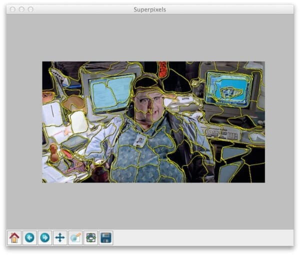
A typical result of applying SLIC to an image looks something like this:

Notice how local regions with similar color and texture distributions are part of the same superpixel group.
That’s a great start.
But how do we access each individual superpixel segmentation?
I’m glad you asked.
Open up your editor, create a file named superpixel_segments.py , and let’s get started:
# import the necessary packages
from skimage.segmentation import slic
from skimage.segmentation import mark_boundaries
from skimage.util import img_as_float
import matplotlib.pyplot as plt
import numpy as np
import argparse
import cv2

# construct the argument parser and parse the arguments
ap = argparse.ArgumentParser()
ap.add_argument("-i", "--image", required = True, help = "Path to the image")
args = vars(ap.parse_args())
Lines 1-8 handle importing the packages we’ll need. We’ll be utilizing scikit-image heavily here, especially for the SLIC implementation. We’ll also be using mark_boundaries , a convenience function that lets us easily visualize the boundaries of the segmentations.
From there, we import matplotlib for plotting, NumPy for numerical processing, argparse for parsing command line arguments, and cv2 for our OpenCV bindings.
Next up, let’s go ahead and parse our command line arguments on Lines 10-13. We’ll need only a single switch --image , which is the path to where our image resides on disk.
Now, let’s perform the actual segmentation:
# load the image and apply SLIC and extract (approximately)
# the supplied number of segments
image = cv2.imread(args["image"])
segments = slic(img_as_float(image), n_segments = 100, sigma = 5)

# show the output of SLIC
fig = plt.figure("Superpixels")
ax = fig.add_subplot(1, 1, 1)
ax.imshow(mark_boundaries(img_as_float(cv2.cvtColor(image, cv2.COLOR_BGR2RGB)), segments))
plt.axis("off")
plt.show()
We start by loading our image on disk on Line 17.
The actual superpixel segmentation takes place on Line 18 by making a call to the slic function. The first argument to this function is our image, represented as a floating point data type rather than the default 8-bit unsigned integer that OpenCV uses. The second argument is the (approximate) number of segmentations we want from slic . And the final parameter is sigma , which is the size of the Gaussian kernel applied prior to the segmentation.
Now that we have our segmentations, we display them on Lines 20-25 using matplotlib .
If you were to execute this code as is, your results would look something like Figure 1 above.
Notice how slic has been applied to construct superpixels in our image. And we can clearly see the “boundaries” of each of these superpixels.
But the real question is “How do we access each individual segmentation?”
It’s actually fairly simple if you know how masks work:
# loop over the unique segment values
for (i, segVal) in enumerate(np.unique(segments)):
	# construct a mask for the segment
	print "[x] inspecting segment %d" % (i)
	mask = np.zeros(image.shape[:2], dtype = "uint8")
	mask[segments == segVal] = 255

	# show the masked region
	cv2.imshow("Mask", mask)
	cv2.imshow("Applied", cv2.bitwise_and(image, image, mask = mask))
	cv2.waitKey(0)
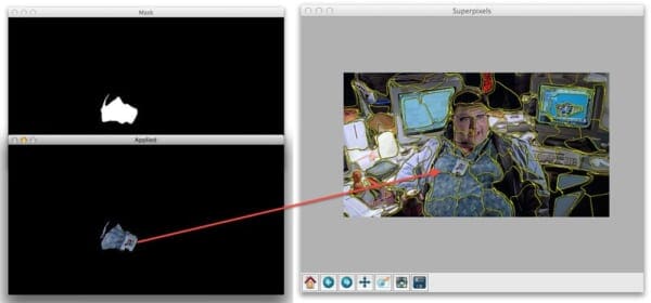
You see, the slic function returns a 2D NumPy array segments with the same width and height as the original image. Furthermore, each segment is represented by a unique integer, meaning that pixels belonging to a particular segmentation will all have the same value in the segments array.
To demonstrate this, let’s start looping over the unique segments values on Line 28.
From there, we construct a mask on Lines 31 and 32. This mask has the same width and height a the original image and has a default value of 0 (black).
However, Line 32 does some pretty important work for us. By stating segments == segVal we find all the indexes, or (x, y) coordinates, in the segments list that have the current segment ID, or segVal . We then pass this list of indexes into the mask and set all these indexes to value of 255 (white).
We can then see the results of our work on Lines 35-37 where we display our mask and the mask applied to our image.
Superpixel Segmentation in Action
To see the results of our work, open a shell and execute the following command:
$ python superpixel_segments.py --image nedry.png
At first, all you’ll see is the superpixel segmentation boundaries, just like above:
But when you close out of that window we’ll start looping over each individual segment. Here are some examples of us accessing each segment:


Nothing to it, right? Now you know how easy it is to access individual superpixel segments using Python, SLIC, and scikit-image.
What's next? We recommend PyImageSearch University.
86+ total classes • 115+ hours hours of on-demand code walkthrough videos • Last updated: April 2026
★★★★★ 4.84 (128 Ratings) • 16,000+ Students Enrolled
I strongly believe that if you had the right teacher you could master computer vision and deep learning.
Do you think learning computer vision and deep learning has to be time-consuming, overwhelming, and complicated? Or has to involve complex mathematics and equations? Or requires a degree in computer science?
That’s not the case.
All you need to master computer vision and deep learning is for someone to explain things to you in simple, intuitive terms. And that’s exactly what I do. My mission is to change education and how complex Artificial Intelligence topics are taught.
If you're serious about learning computer vision, your next stop should be PyImageSearch University, the most comprehensive computer vision, deep learning, and OpenCV course online today. Here you’ll learn how to successfully and confidently apply computer vision to your work, research, and projects. Join me in computer vision mastery.
Inside PyImageSearch University you'll find:
- ✓ 86+ courses on essential computer vision, deep learning, and OpenCV topics
- ✓ 86 Certificates of Completion
- ✓ 115+ hours hours of on-demand video
- ✓ Brand new courses released regularly, ensuring you can keep up with state-of-the-art techniques
- ✓ Pre-configured Jupyter Notebooks in Google Colab
- ✓ Run all code examples in your web browser — works on Windows, macOS, and Linux (no dev environment configuration required!)
- ✓ Access to centralized code repos for all 540+ tutorials on PyImageSearch
- ✓ Easy one-click downloads for code, datasets, pre-trained models, etc.
- ✓ Access on mobile, laptop, desktop, etc.
Summary
In this blog post I showed you how to utilize the Simple Linear Iterative Clustering (SLIC) algorithm to perform superpixel segmentation.
From there, I provided code that allows you to access each individual segmentation produced by the algorithm.
So now that you have each of these segmentations, what do you do?
To start, you could look into graph representations across regions of the image. Another option would be to extract features from each of the segmentations which you could later utilize to construct a bag-of-visual-words. This bag-of-visual-words model would be useful for training a machine learning classifier or building a Content-Based Image Retrieval system. But more on that later…
Anyway, I hope you enjoyed this article! This certainly won’t be the last time we discuss superpixel segmentations.
And if you’re interested in downloading the code to this blog post, just enter your email address in the form below and I’ll email you the code and example images. And I’ll also be sure to notify you when new awesome PyImageSearch content is released!

Download the Source Code and FREE 17-page Resource Guide
Enter your email address below to get a .zip of the code and a FREE 17-page Resource Guide on Computer Vision, OpenCV, and Deep Learning. Inside you'll find my hand-picked tutorials, books, courses, and libraries to help you master CV and DL!

