Training an object detector from scratch in PyTorch

In this tutorial, you will learn how to train a custom object detector from scratch using PyTorch.

This lesson is part 2 of a 3-part series on advanced PyTorch techniques:

1. Training a DCGAN in PyTorch (last week’s tutorial)
2. Training an object detector from scratch in PyTorch (today’s tutorial)
3. U-Net: Training Image Segmentation Models in PyTorch (next week’s blog post)

Since my childhood, the idea of artificial intelligence (AI) has fascinated me (like every other kid). But, of course, the concept of AI that I had was vastly different from what it actually was, unquestionably due to pop culture. Until the end of my teenage years, I firmly believed that the unchecked growth of AI would lead to something like the T-800 (the terminator from The Terminator). Fortunately, the actual scenario can be better explained using Figure 1:

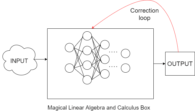
Don’t get me wrong, though. Machine Learning may be a bunch of matrices and calculus coalesced together, but the sheer amount of things we can do with these can be best described by a single word: limitless.

One such application, which always intrigued me, was Object Detection. Pouring in image data to get labels was one thing, but making our model learn where the label is? That’s a whole different ball game, something right out of some espionage movie. And that is exactly what we’ll be going through today!

In today’s tutorial, we’ll learn how to train our very own object detector from scratch in PyTorch. This blog will help you:

• Understand the intuition behind Object Detection
• Understand the step-by-step approach to building your own Object Detector
• Learn how to fine-tune parameters to get ideal results

To learn how to train an object detector from scratch in Pytorch, just keep reading.

Training an Object Detector from scratch in PyTorch

Much before the power deep learning algorithms of today existed, Object Detection was a domain that was extensively worked on throughout history. From the late 1990s to the early 2020s, many new ideas were proposed, which are still used as benchmarks for deep learning algorithms to this day. Unfortunately, back then, researchers didn’t have much computation power at their disposal, so most of these techniques relied on lots of additional mathematics to reduce compute time. Thankfully, we wouldn’t be facing that problem.

Our Approach to Object Detection

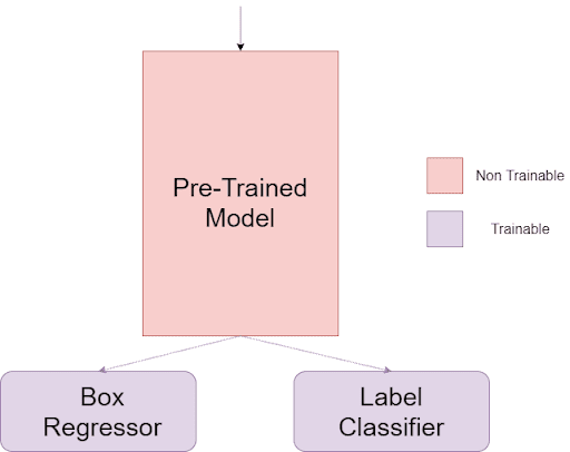
Let’s first understand the intuition behind Object Detection. The approach we are going to take is quite similar to training a simple classifier. The weights of the classifier keep changing until it outputs the correct labels for a given dataset and reduces loss. We will be doing the exact same thing for today’s task, except our model will output 5 values, 4 of them being the coordinates of the bounding box surrounding our object. The 5th value is the label of the object being detected. Notice the architecture in Figure 2.

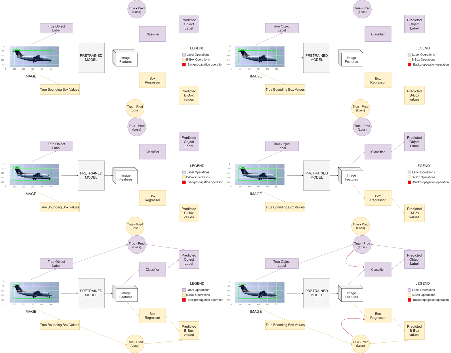
The main model will branch into two subsets: the regressor and the classifier. The former will output the bounding box’s starting and ending coordinates, while the latter will output the object label. The combined losses generated by these 5 values will serve in our backpropagation. Quite a simple way to start, isn’t it?

Of course, through the years, several powerful algorithms took over the Object Detection domain, like R-CNN and YOLO. But our approach will serve as a reasonable starting point to wrap your head around the basic idea behind Object Detection!

Configuring your development environment

To follow this guide, first and foremost, you need to have PyTorch installed in your system. To access PyTorch’s own set of models for vision computing, you will also need to have Torchvision in your system. For some array and storage operations, we have employed the use of numpy. We are also using the imutils package for data handling. For our plots, we will be using matplotlib. For better tracking of our model training, we’ll be using tqdm, and finally, we’ll be needing OpenCV in our system!

Luckily, all of the above-mentioned packages are pip-installable!

$ pip install opencv-contrib-python
$ pip install torch
$ pip install torchvision
$ pip install imutils
$ pip install matplotlib
$ pip install numpy
$ pip install tqdm

If you need help configuring your development environment for OpenCV, I highly recommend that you read my pip install OpenCV guide — it will have you up and running in a matter of minutes.

Having problems configuring your development environment?

All that said, are you:

• Short on time?
• Learning on your employer’s administratively locked system?
• Wanting to skip the hassle of fighting with the command line, package managers, and virtual environments?
• Ready to run the code right now on your Windows, macOS, or Linux system?

Then join PyImageSearch University today!

Gain access to Jupyter Notebooks for this tutorial and other PyImageSearch guides that are pre-configured to run on Google Colab’s ecosystem right in your web browser! No installation required.

And best of all, these Jupyter Notebooks will run on Windows, macOS, and Linux!

Project structure

We first need to review our project directory structure.

Start by accessing the “Downloads” section of this tutorial to retrieve the source code and example images.

From there, take a look at the directory structure:

!tree .
.
├── dataset.zip
├── output
│   ├── detector.pth
│   ├── le.pickle
│   ├── plots
│   │   └── training.png
│   └── test_paths.txt
├── predict.py
├── pyimagesearch
│   ├── bbox_regressor.py
│   ├── config.py
│   ├── custom_tensor_dataset.py
│   └── __init__.py
└── train.py

The first item in the directory is dataset.zip. This zip file contains the complete dataset (Images, labels, and bounding boxes). More about it in a later section.

Next, we have the output directory. This directory is where all our saved models, results, and other important requirements are dumped.

There are two scripts in the parent directory:

• train.py: used to train our object detector
• predict.py: used to draw inference from our model and see the object detector in action

Lastly, we have the most important directory, the pyimagesearch directory. It houses 3 very important scripts.

• bbox_regressor.py: houses the complete object detector architecture
• config.py: contains the configuration of the end-to-end training and inference pipeline
• custom_tensor_dataset.py: contains a custom class for data preparation

That concludes the review of our project directory.

Configuring the prerequisites for Object Detection

Our first task is to configure several hyperparameters we’ll be using throughout the project. For that, let’s hop into the pyimagesearch folder and open the config.py script.

# import the necessary packages
import torch
import os

# define the base path to the input dataset and then use it to derive
# the path to the input images and annotation CSV files
BASE_PATH = "dataset"
IMAGES_PATH = os.path.sep.join([BASE_PATH, "images"])
ANNOTS_PATH = os.path.sep.join([BASE_PATH, "annotations"])

# define the path to the base output directory
BASE_OUTPUT = "output"

# define the path to the output model, label encoder, plots output
# directory, and testing image paths
MODEL_PATH = os.path.sep.join([BASE_OUTPUT, "detector.pth"])
LE_PATH = os.path.sep.join([BASE_OUTPUT, "le.pickle"])
PLOTS_PATH = os.path.sep.join([BASE_OUTPUT, "plots"])
TEST_PATHS = os.path.sep.join([BASE_OUTPUT, "test_paths.txt"])

We start by defining several paths which we will later use. Then on Lines 7-12, we define paths for our datasets (Images and annotations) and output. Next, we create separate paths for our detector and label encoder, followed by paths for our plots and testing images (Lines 16-19).

# determine the current device and based on that set the pin memory
# flag
DEVICE = "cuda" if torch.cuda.is_available() else "cpu"
PIN_MEMORY = True if DEVICE == "cuda" else False

# specify ImageNet mean and standard deviation
MEAN = [0.485, 0.456, 0.406]
STD = [0.229, 0.224, 0.225]

# initialize our initial learning rate, number of epochs to train
# for, and the batch size
INIT_LR = 1e-4
NUM_EPOCHS = 20
BATCH_SIZE = 32

# specify the loss weights
LABELS = 1.0
BBOX = 1.0

Since we are training an object detector, it’s advisable to train on a GPU instead of a CPU since the computations are more complex. Hence, we set our PyTorch device to CUDA if a CUDA-compatible GPU is available in our system (Lines 23 and 24).

We will, of course, be using PyTorch’s transforms during our dataset preparation. Hence we specify the mean and standard deviation values (Lines 27 and 28). The three values represent the channel-wise, width-wise, and height-wise mean and standard deviation, respectively. Finally, we initialize hyperparameters like learning rate, epochs, batch size, and Loss weights for our model (Lines 32-38).

Creating the Custom Object Detection Data processor

Let’s have a look at our data directory.

!tree . 
.
├── dataset
│   ├── annotations
│   └── images
│       ├── airplane
│       ├── face
│       └── motorcycle

The dataset subdivides into two folders: annotations (which contains CSV files of bounding box start and end points) and images (which are further divided into three folders, each representing the classes we’ll be using today).

Since we’ll use PyTorch’s own DataLoader, it’s important to preprocess the data in a way that the DataLoader will accept. The custom_tensor_dataset.py script will do exactly that.

# import the necessary packages
from torch.utils.data import Dataset

class CustomTensorDataset(Dataset):
	# initialize the constructor
	def __init__(self, tensors, transforms=None):
		self.tensors = tensors
		self.transforms = transforms

We have created a custom class, CustomTensorDataset, which inherits from the torch.utils.data.Dataset class (Line 4). This way, we can configure the internal functions to our needs while retaining the core properties of the torch.utils.data.Dataset class.

On Lines 6-8, the constructor function __init__ is created. The constructor takes in two arguments:

• tensors: A tuple of three tensors, namely the image, label, and the bounding box coordinates.
• transforms: A torchvision.transforms instance which will be used to process the image.

	def __getitem__(self, index):
		# grab the image, label, and its bounding box coordinates
		image = self.tensors[0][index]
		label = self.tensors[1][index]
		bbox = self.tensors[2][index]

		# transpose the image such that its channel dimension becomes
		# the leading one
		image = image.permute(2, 0, 1)

		# check to see if we have any image transformations to apply
		# and if so, apply them
		if self.transforms:
			image = self.transforms(image)

		# return a tuple of the images, labels, and bounding
		# box coordinates
		return (image, label, bbox)

Since we are using a custom class, we will override the parent (Dataset) class’s methods. So, the __getitem__ method is altered according to our needs. But, first, the tensor tuple is unpacked into its constituents (Lines 12-14).

The image tensor is originally in the form Height × Width × Channels. However, all PyTorch models need their input to be “channel first.” Accordingly, the image.permute method rearranges the image tensor (Line 18).

We add a check for the torchvision.transforms instance on Lines 22 and 23. If the check yields true, the image is passed through the transform instance. After this, the __getitem__ method returns the image, label, and bounding boxes.

	def __len__(self):
		# return the size of the dataset
		return self.tensors[0].size(0)

The second method that we’ll override is the __len__ method. It returns the size of the image dataset tensor (Lines 29-31). This concludes the custom_tensor_dataset.py script.

Building the Objection Detection Architecture

Coming to the model we’ll be needing for this project, we need to keep two things in mind. First, to avoid additional hassle and for efficient feature extraction, we’ll use a pre-trained model to act as the base model. Second, the base model will then be split into two parts; the box regressor and the label classifier. Both of these will be individual model entities.

The second thing to remember is that only the box regressor and the label classifier will have trainable weights. The weights of the pre-trained model will be left untouched, as shown in Figure 4.

With this in mind, let’s hop into bbox_regressor.py!

# import the necessary packages
from torch.nn import Dropout
from torch.nn import Identity
from torch.nn import Linear
from torch.nn import Module
from torch.nn import ReLU
from torch.nn import Sequential
from torch.nn import Sigmoid

class ObjectDetector(Module):
	def __init__(self, baseModel, numClasses):
		super(ObjectDetector, self).__init__()

		# initialize the base model and the number of classes
		self.baseModel = baseModel
		self.numClasses = numClasses

For the custom model ObjectDetector, we’ll use torch.nn.Module as the parent class (Line 10). For the constructor function __init__, there are two external arguments; the base model and the number of labels (Lines 11-16).

		# build the regressor head for outputting the bounding box
		# coordinates
		self.regressor = Sequential(
			Linear(baseModel.fc.in_features, 128),
			ReLU(),
			Linear(128, 64),
			ReLU(),
			Linear(64, 32),
			ReLU(),
			Linear(32, 4),
			Sigmoid()
		)

Moving on to the regressor, keep in mind that our end goal is to produce 4 separate values: the starting x-axis value, the starting y-axis value, the ending x-axis value, and the ending y-axis value. The first Linear layer inputs the fully connected layer of the base model with an output size set to 128 (Line 21).

This is followed by a few Linear and ReLU layers (Lines 22-27), finally ending with a Linear layer which outputs 4 values followed by a Sigmoid layer (Line 28).

		# build the classifier head to predict the class labels
		self.classifier = Sequential(
			Linear(baseModel.fc.in_features, 512),
			ReLU(),
			Dropout(),
			Linear(512, 512),
			ReLU(),
			Dropout(),
			Linear(512, self.numClasses)
		)

		# set the classifier of our base model to produce outputs
		# from the last convolution block
		self.baseModel.fc = Identity()

The next step is the classifier for the object label. In the Regressor, we take the base model’s fully connected layer’s feature size and plug it into the first Linear layer (Line 33). This is followed by repeating the ReLU, Dropout, and Linear layers (Lines 34-40). The Dropout layers are generally used to help spread generalization and prevent overfitting.

The final step of the initialization is to make the base model’s fully connected layer into an Identity layer, which means it’ll mirror the outputs produced by the convolution block right before it (Line 44).

 	def forward(self, x):
		# pass the inputs through the base model and then obtain
		# predictions from two different branches of the network
		features = self.baseModel(x)
		bboxes = self.regressor(features)
		classLogits = self.classifier(features)

		# return the outputs as a tuple
		return (bboxes, classLogits)

Next comes the forward step (Line 46). We simply take the output of the base model and pass it through the regressor and the classifier (Lines 49-51).

With that, we finish designing the architecture of our object detector.

Training the Object Detection Model

Just one more step remaining before we can see the object detector in action. So let’s hop over to the train.py script and train the model!

# USAGE
# python train.py

# import the necessary packages
from pyimagesearch.bbox_regressor import ObjectDetector
from pyimagesearch.custom_tensor_dataset import CustomTensorDataset
from pyimagesearch import config
from sklearn.preprocessing import LabelEncoder
from torch.utils.data import DataLoader
from torchvision import transforms
from torch.nn import CrossEntropyLoss
from torch.nn import MSELoss
from torch.optim import Adam
from torchvision.models import resnet50
from sklearn.model_selection import train_test_split
from imutils import paths
from tqdm import tqdm
import matplotlib.pyplot as plt
import numpy as np
import pickle
import torch
import time
import cv2
import os

# initialize the list of data (images), class labels, target bounding
# box coordinates, and image paths
print("[INFO] loading dataset...")
data = []
labels = []
bboxes = []
imagePaths = []

After importing the necessary packages, we create empty lists for our data, labels, bounding boxes, and image paths (Lines 29-32).

Now it’s time for some data pre-processing.

# loop over all CSV files in the annotations directory
for csvPath in paths.list_files(config.ANNOTS_PATH, validExts=(".csv")):
	# load the contents of the current CSV annotations file
	rows = open(csvPath).read().strip().split("\n")

	# loop over the rows
	for row in rows:
		# break the row into the filename, bounding box coordinates,
		# and class label
		row = row.split(",")
		(filename, startX, startY, endX, endY, label) = row

		# derive the path to the input image, load the image (in
		# OpenCV format), and grab its dimensions
		imagePath = os.path.sep.join([config.IMAGES_PATH, label,
			filename])
		image = cv2.imread(imagePath)
		(h, w) = image.shape[:2]

		# scale the bounding box coordinates relative to the spatial
		# dimensions of the input image
		startX = float(startX) / w
		startY = float(startY) / h
		endX = float(endX) / w
		endY = float(endY) / h

		# load the image and preprocess it
		image = cv2.imread(imagePath)
		image = cv2.cvtColor(image, cv2.COLOR_BGR2RGB)
		image = cv2.resize(image, (224, 224))

		# update our list of data, class labels, bounding boxes, and
		# image paths
		data.append(image)
		labels.append(label)
		bboxes.append((startX, startY, endX, endY))
		imagePaths.append(imagePath)

On Line 35, we start looping over all available CSVs in the directory. Opening the CSVs, we then begin looping over the rows to split the data (Lines 37-44).

After splitting the row values into a tuple of individual values, we first single out the image path (Line 48). Then, we use OpenCV to read the image and get its height and width (Lines 50 and 51).

The height and width values are then used to scale the bounding box coordinates to the range of 0 and 1 (Lines 55-58).

Next, we load the image and do some slight preprocessing (Lines 61-63).

The empty lists are then updated with the unpacked values, and the process repeats as each iteration passes (Lines 67-70).

# convert the data, class labels, bounding boxes, and image paths to
# NumPy arrays
data = np.array(data, dtype="float32")
labels = np.array(labels)
bboxes = np.array(bboxes, dtype="float32")
imagePaths = np.array(imagePaths)

# perform label encoding on the labels
le = LabelEncoder()
labels = le.fit_transform(labels)

For faster processing of data, the lists are converted into numpy arrays (Lines 74-77). Since the labels are in string format, we use scikit-learn’s LabelEncoder to transform them into their respective indices (Lines 80 and 81).

# partition the data into training and testing splits using 80% of
# the data for training and the remaining 20% for testing
split = train_test_split(data, labels, bboxes, imagePaths,
	test_size=0.20, random_state=42)

# unpack the data split
(trainImages, testImages) = split[:2]
(trainLabels, testLabels) = split[2:4]
(trainBBoxes, testBBoxes) = split[4:6]
(trainPaths, testPaths) = split[6:]

Using another handy scikit-learn tool called train_test_split, we part the data into training and test sets, keeping an 80-20 ratio (Lines 85 and 86). Since the split will apply to all the arrays passed into the train_test_split function, we can unpack them into tuples using simple row slicing (Lines 89-92).

# convert NumPy arrays to PyTorch tensors
(trainImages, testImages) = torch.tensor(trainImages),\
	torch.tensor(testImages)
(trainLabels, testLabels) = torch.tensor(trainLabels),\
	torch.tensor(testLabels)
(trainBBoxes, testBBoxes) = torch.tensor(trainBBoxes),\
	torch.tensor(testBBoxes)

# define normalization transforms
transforms = transforms.Compose([
	transforms.ToPILImage(),
	transforms.ToTensor(),
	transforms.Normalize(mean=config.MEAN, std=config.STD)
])

The unpacked train and test data, labels, and bounding boxes are then converted into PyTorch tensors from the numpy format (Lines 95-100). Next, we proceed to create a torchvision.transforms instance to easily process the dataset (Lines 103-107). Through this, the dataset will also get normalized using the mean and standard deviation values defined in config.py.

# convert NumPy arrays to PyTorch datasets
trainDS = CustomTensorDataset((trainImages, trainLabels, trainBBoxes),
	transforms=transforms)
testDS = CustomTensorDataset((testImages, testLabels, testBBoxes),
	transforms=transforms)
print("[INFO] total training samples: {}...".format(len(trainDS)))
print("[INFO] total test samples: {}...".format(len(testDS)))

# calculate steps per epoch for training and validation set
trainSteps = len(trainDS) // config.BATCH_SIZE
valSteps = len(testDS) // config.BATCH_SIZE

# create data loaders
trainLoader = DataLoader(trainDS, batch_size=config.BATCH_SIZE,
	shuffle=True, num_workers=os.cpu_count(), pin_memory=config.PIN_MEMORY)
testLoader = DataLoader(testDS, batch_size=config.BATCH_SIZE,
	num_workers=os.cpu_count(), pin_memory=config.PIN_MEMORY)

Remember, in the custom_tensor_dataset.py script, we created a custom Dataset class to cater to our exact needs. As of now, our required entities are just tensors. So, to turn them into a PyTorch DataLoader accepted format, we create training and testing instances of the CustomTensorDataset class, passing the images, labels, and the bounding boxes as arguments (Lines 110-113).

On Lines 118 and 119, the steps per epoch values are calculated using the length of the datasets and the batch size value set in config.py.

Finally, we pass the CustomTensorDataset instances through the DataLoader and create the train and test Data loaders (Lines 122-125).

# write the testing image paths to disk so that we can use then
# when evaluating/testing our object detector
print("[INFO] saving testing image paths...")
f = open(config.TEST_PATHS, "w")
f.write("\n".join(testPaths))
f.close()

# load the ResNet50 network
resnet = resnet50(pretrained=True)

# freeze all ResNet50 layers so they will *not* be updated during the
# training process
for param in resnet.parameters():
	param.requires_grad = False

Since we’ll be using the test image paths for evaluation later, it’s written to the disk (Lines 129-132).

For the base model in our architecture, we’ll be using a pre-trained resnet50 (Line 135). However, as mentioned before, the weights of the base model will be left untouched. Hence, we freeze the weights (Lines 139 and 140).

# create our custom object detector model and flash it to the current
# device
objectDetector = ObjectDetector(resnet, len(le.classes_))
objectDetector = objectDetector.to(config.DEVICE)

# define our loss functions
classLossFunc = CrossEntropyLoss()
bboxLossFunc = MSELoss()

# initialize the optimizer, compile the model, and show the model
# summary
opt = Adam(objectDetector.parameters(), lr=config.INIT_LR)
print(objectDetector)

# initialize a dictionary to store training history
H = {"total_train_loss": [], "total_val_loss": [], "train_class_acc": [],
	 "val_class_acc": []}

With the model prerequisites complete, we create our custom model instance and load it to the current device (Lines 144 and 145). For the classifier loss, Cross-Entropy loss is being used, while for the Box Regressor, we are sticking to Mean squared error loss (Lines 148 and 149). On Line 153, Adam is set as the Object Detector optimizer. To track the training loss and other metrics, a dictionary H is initialized on Lines 157 and 158.

# loop over epochs
print("[INFO] training the network...")
startTime = time.time()
for e in tqdm(range(config.NUM_EPOCHS)):
	# set the model in training mode
	objectDetector.train()

	# initialize the total training and validation loss
	totalTrainLoss = 0
	totalValLoss = 0

	# initialize the number of correct predictions in the training
	# and validation step
	trainCorrect = 0
	valCorrect = 0

For training speed assessment, the start time is noted (Line 162). Looping over the number of epochs, we first set the object detector to training mode (Line 165) and initialize the losses and number of correct predictions (Lines 168-174).

	# loop over the training set
	for (images, labels, bboxes) in trainLoader:
		# send the input to the device
		(images, labels, bboxes) = (images.to(config.DEVICE),
			labels.to(config.DEVICE), bboxes.to(config.DEVICE))

		# perform a forward pass and calculate the training loss
		predictions = objectDetector(images)
		bboxLoss = bboxLossFunc(predictions[0], bboxes)
		classLoss = classLossFunc(predictions[1], labels)
		totalLoss = (config.BBOX * bboxLoss) + (config.LABELS * classLoss)

		# zero out the gradients, perform the backpropagation step,
		# and update the weights
		opt.zero_grad()
		totalLoss.backward()
		opt.step()

		# add the loss to the total training loss so far and
		# calculate the number of correct predictions
		totalTrainLoss += totalLoss
		trainCorrect += (predictions[1].argmax(1) == labels).type(
			torch.float).sum().item()

Looping over the train data loader, we first load the images, labels, and bounding boxes to the device in use (Lines 179 and 180). Next, we plug the images into our Object Detector and store the predictions (Line 183). Finally, since the model will give two predictions (one for the label and one for the bounding box), we index those out and calculate those losses, respectively (Lines 183-185).

The combined value of both the losses will act as the total loss for the architecture. We multiply the respective loss weights for the bounding box loss and the label loss defined in config.py to the losses and sum them up (Line 186).

With the help of PyTorch’s automatic gradient functionality, we simply reset the gradients, calculate the weights due to the loss generated, and update the parameter based on the gradient of the current step (Lines 190-192). It is important to reset the gradients because the backward function keeps accumulating the gradients altogether. Since we only want the gradient pertaining to the current step, the opt.zero_grad flushes out the previous values.

On Lines 196-198, we update the loss values and correct predictions.

	# switch off autograd
	with torch.no_grad():
		# set the model in evaluation mode
		objectDetector.eval()

		# loop over the validation set
		for (images, labels, bboxes) in testLoader:
			# send the input to the device
			(images, labels, bboxes) = (images.to(config.DEVICE),
				labels.to(config.DEVICE), bboxes.to(config.DEVICE))

			# make the predictions and calculate the validation loss
			predictions = objectDetector(images)
			bboxLoss = bboxLossFunc(predictions[0], bboxes)
			classLoss = classLossFunc(predictions[1], labels)
			totalLoss = (config.BBOX * bboxLoss) + \
				(config.LABELS * classLoss)
			totalValLoss += totalLoss

			# calculate the number of correct predictions
			valCorrect += (predictions[1].argmax(1) == labels).type(
				torch.float).sum().item()

Moving on to the model evaluation, we’ll first turn off automatic gradients and switch to the evaluation mode of the object detector (Lines 201-203). Then, looping over the test data, we’ll repeat the same process as done in training apart from updating the weights (Lines 212-214).

The combined loss is calculated in the same manner as the training step (Lines 215 and 216). Consequently, the total loss value and correct predictions are updated (Lines 217-221).

	# calculate the average training and validation loss
	avgTrainLoss = totalTrainLoss / trainSteps
	avgValLoss = totalValLoss / valSteps

	# calculate the training and validation accuracy
	trainCorrect = trainCorrect / len(trainDS)
	valCorrect = valCorrect / len(testDS)

	# update our training history
	H["total_train_loss"].append(avgTrainLoss.cpu().detach().numpy())
	H["train_class_acc"].append(trainCorrect)
	H["total_val_loss"].append(avgValLoss.cpu().detach().numpy())
	H["val_class_acc"].append(valCorrect)

	# print the model training and validation information
	print("[INFO] EPOCH: {}/{}".format(e + 1, config.NUM_EPOCHS))
	print("Train loss: {:.6f}, Train accuracy: {:.4f}".format(
		avgTrainLoss, trainCorrect))
	print("Val loss: {:.6f}, Val accuracy: {:.4f}".format(
		avgValLoss, valCorrect))
endTime = time.time()
print("[INFO] total time taken to train the model: {:.2f}s".format(
	endTime - startTime))

After one epoch, the average batchwise training and testing losses are calculated on Lines 224 and 225. We also calculate the training and testing accuracies of the epoch using the number of correct predictions (Lines 228 and 229).

Following the calculations, all values are logged in the model history dictionary H (Lines 232-235), while the end time is calculated to see how long the training took and after exiting the loop (Line 243).

# serialize the model to disk
print("[INFO] saving object detector model...")
torch.save(objectDetector, config.MODEL_PATH)

# serialize the label encoder to disk
print("[INFO] saving label encoder...")
f = open(config.LE_PATH, "wb")
f.write(pickle.dumps(le))
f.close()

# plot the training loss and accuracy
plt.style.use("ggplot")
plt.figure()
plt.plot(H["total_train_loss"], label="total_train_loss")
plt.plot(H["total_val_loss"], label="total_val_loss")
plt.plot(H["train_class_acc"], label="train_class_acc")
plt.plot(H["val_class_acc"], label="val_class_acc")
plt.title("Total Training Loss and Classification Accuracy on Dataset")
plt.xlabel("Epoch #")
plt.ylabel("Loss/Accuracy")
plt.legend(loc="lower left")

# save the training plot
plotPath = os.path.sep.join([config.PLOTS_PATH, "training.png"])
plt.savefig(plotPath)

Since we’ll use the object detector for inference, we save it to the disk (Line 249). We also save the label encoder that was created so that the pattern remains unchanged (Lines 253-255)

To assess the model training, we plot all the metrics stored in the model history dictionary H (Lines 258-271).

This ends the model training. Next, let’s look at how well the object detector trained!

Assessing the Object Detection Training

Since the bulk of the model will have its weights unchanged, the training shouldn’t take long. First, let’s take a look at some of the training epochs.

[INFO] training the network...
  0%|          | 0/20 [00:00<?,  
  5%|▌         | 1/20 [00:16<05:08, 16.21s/it][INFO] EPOCH: 1/20
Train loss: 0.874699, Train accuracy: 0.7608
Val loss: 0.360270, Val accuracy: 0.9902
 10%|█         | 2/20 [00:31<04:46, 15.89s/it][INFO] EPOCH: 2/20
Train loss: 0.186642, Train accuracy: 0.9834
Val loss: 0.052412, Val accuracy: 1.0000
 15%|█▌        | 3/20 [00:47<04:28, 15.77s/it][INFO] EPOCH: 3/20
Train loss: 0.066982, Train accuracy: 0.9883
...
 85%|████████▌ | 17/20 [04:27<00:47, 15.73s/it][INFO] EPOCH: 17/20
Train loss: 0.011934, Train accuracy: 0.9975
Val loss: 0.004053, Val accuracy: 1.0000
 90%|█████████ | 18/20 [04:43<00:31, 15.67s/it][INFO] EPOCH: 18/20
Train loss: 0.009135, Train accuracy: 0.9975
Val loss: 0.003720, Val accuracy: 1.0000
 95%|█████████▌| 19/20 [04:58<00:15, 15.66s/it][INFO] EPOCH: 19/20
Train loss: 0.009403, Train accuracy: 0.9982
Val loss: 0.003248, Val accuracy: 1.0000
100%|██████████| 20/20 [05:14<00:00, 15.73s/it][INFO] EPOCH: 20/20
Train loss: 0.006543, Train accuracy: 0.9994
Val loss: 0.003041, Val accuracy: 1.0000
[INFO] total time taken to train the model: 314.68s

We see that the model reached astounding accuracies at 0.9994 and 1.0000 for training and validation, respectively. Let’s see the epoch-wise variation on the training plot Figure 5!

The model reached saturation levels fairly quickly in both the training and validation values. Now it’s time to see the object detector in action!

Drawing Inference from the Object Detector

The final step in this journey is at the predict.py script. Here, we will individually loop over the test images and draw bounding boxes with our predicted values.

# USAGE
# python predict.py --input dataset/images/face/image_0131.jpg

# import the necessary packages
from pyimagesearch import config
from torchvision import transforms
import mimetypes
import argparse
import imutils
import pickle
import torch
import cv2

# construct the argument parser and parse the arguments
ap = argparse.ArgumentParser()
ap.add_argument("-i", "--input", required=True,
	help="path to input image/text file of image paths")
args = vars(ap.parse_args())

The argparse module is used to write user-friendly command line interface commands. On Lines 15-18, we construct an argument parser to help the user select the test image.

# determine the input file type, but assume that we're working with
# single input image
filetype = mimetypes.guess_type(args["input"])[0]
imagePaths = [args["input"]]

# if the file type is a text file, then we need to process *multiple*
# images
if "text/plain" == filetype:
	# load the image paths in our testing file
	imagePaths = open(args["input"]).read().strip().split("\n")

We follow the argument parsing with steps to deal with any kind of input the user proceeds to give. On Lines 22 and 23, the imagePaths variable is set to deal with a single input image, while on Lines 27-29, the event of multiple images is dealt with.

# load our object detector, set it evaluation mode, and label
# encoder from disk
print("[INFO] loading object detector...")
model = torch.load(config.MODEL_PATH).to(config.DEVICE)
model.eval()
le = pickle.loads(open(config.LE_PATH, "rb").read())

# define normalization transforms
transforms = transforms.Compose([
	transforms.ToPILImage(),
	transforms.ToTensor(),
	transforms.Normalize(mean=config.MEAN, std=config.STD)
])

The model which was trained using the train.py script is called for evaluation (Lines 34 and 35). Similarly, the label encoder stored using the aforementioned script is loaded (Line 36). Since we’ll be needing to process the data again, another torchvision.transforms instance is created, having the same arguments as the ones used during training.

# loop over the images that we'll be testing using our bounding box
# regression model
for imagePath in imagePaths:
	# load the image, copy it, swap its colors channels, resize it, and
	# bring its channel dimension forward
	image = cv2.imread(imagePath)
	orig = image.copy()
	image = cv2.cvtColor(image, cv2.COLOR_BGR2RGB)
	image = cv2.resize(image, (224, 224))
	image = image.transpose((2, 0, 1))

	# convert image to PyTorch tensor, normalize it, flash it to the
	# current device, and add a batch dimension
	image = torch.from_numpy(image)
	image = transforms(image).to(config.DEVICE)
	image = image.unsqueeze(0)

Looping over the test images, we read the image and apply some preprocessing to it (Lines 50-54). This is done since our image needs to be plugged into the object detector again.

We proceed to turn the image into a tensor, apply the torchvision.transforms instance to it, and add a batching dimension to it (Lines 58-60). Our test image is now ready to be plugged into the object detector.

	# predict the bounding box of the object along with the class
	# label
	(boxPreds, labelPreds) = model(image)
	(startX, startY, endX, endY) = boxPreds[0]

	# determine the class label with the largest predicted
	# probability
	labelPreds = torch.nn.Softmax(dim=-1)(labelPreds)
	i = labelPreds.argmax(dim=-1).cpu()
	label = le.inverse_transform(i)[0]

First, the predictions from the model are obtained (Line 64). We proceed to unpack the bounding box values from the boxPreds variable (Line 65).

A simple softmax function on the Label prediction will give us a better picture of the values corresponding to the classes. For that purpose, we use PyTorch’s own torch.nn.Softmax on Line 69. Isolating the index with argmax, we plug it in the Label encoder le and use inverse_transform (Index to value) to get the name of the label (Lines 69-71).

	# resize the original image such that it fits on our screen, and
	# grab its dimensions
	orig = imutils.resize(orig, width=600)
	(h, w) = orig.shape[:2]

	# scale the predicted bounding box coordinates based on the image
	# dimensions
	startX = int(startX * w)
	startY = int(startY * h)
	endX = int(endX * w)
	endY = int(endY * h)

	# draw the predicted bounding box and class label on the image
	y = startY - 10 if startY - 10 > 10 else startY + 10
	cv2.putText(orig, label, (startX, y), cv2.FONT_HERSHEY_SIMPLEX,
		0.65, (0, 255, 0), 2)
	cv2.rectangle(orig, (startX, startY), (endX, endY),
		(0, 255, 0), 2)

	# show the output image 
	cv2.imshow("Output", orig)
	cv2.waitKey(0)

On Line 75, we have resized the original image to fit our screen. The height and width of the resized image are then stored, to scale the predicted bounding box values based on the image (Lines 76-83). This is done because we had scaled down the annotations to the range 0 and 1 before fitting them to the model. Hence, all outputs would have to be scaled up for display purposes.

While displaying the bounding box, the label name will also be shown on top of it. For that purpose, we set up the y-axis value for our text on Line 86. Using OpenCV’s putText function, we set up the label displayed on the image (Lines 87 and 88).

Finally, we use OpenCV’s rectangle method to create the bounding box on the image (Lines 89 and 90). Since we have the starting x-axis, starting y-axis, ending x-axis, and ending y-axis values, it’s very easy to create a rectangle from them. This rectangle will surround our object.

This concludes our inference script. Let’s take a look at the results!

Object Detection in Action

Let’s see how our object detector fared, using one image from each class. We first use an image of an airplane (Figure 6), followed by an image under faces (Figure 7), and an image belonging to the motorcycle class (Figure 8).

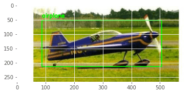
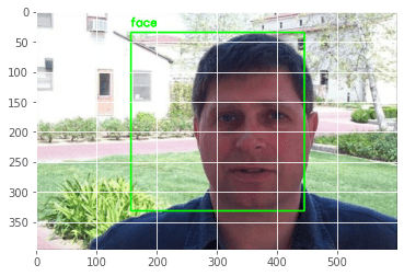
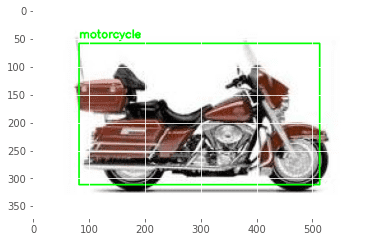
As it turns out, the accuracy values of our model weren’t lying. Not only did our model correctly guess the label, but the bounding boxes produced are also almost perfect!

With such precise detection and results, we can all agree that our little project was a success, can’t we?

Summary

While writing this Object Detection tutorial, I realized a few things in retrospect.

To be very honest, I had never liked using pre-trained models for my projects. It would feel that my work isn’t my work anymore. Obviously, that turned out to be a stupid notion, solidified with the fact that my first one-shot face classifier said that my best friend and I were the same people (believe me, we don’t look remotely similar).

I would say this tutorial served as a beautiful example of what happens when you have a well-trained feature extractor. Not only did we save time, but the end results were also brilliant. Take Figures 6 and 8 as examples. The predicted bounding boxes have minimal error.

Of course, this doesn’t mean there isn’t room for improvement. In Figure 7, the image has many elements, yet the object detector has managed to capture the general area of the object. However, it could have been more compact. We urge you to tinker around with the parameters to see if your results are better!

That being said, Object Detection really plays a vital role in our world today. Automated Traffic, face detections, self-driving cars are just a few of the real-world applications where Object Detection thrives. Each year, algorithms are designed to make the process faster and more compact. We have reached a stage where algorithms can concurrently detect all objects inside scenes of a video! I hope this tutorial has piqued your curiosity toward uncovering the intricacies of this domain.

To download the source code to this post (and be notified when future tutorials are published here on PyImageSearch), simply enter your email address in the form below!