Image Gradients with OpenCV (Sobel and Scharr)

In this tutorial, you will learn about image gradients and how to compute Sobel gradients and Scharr gradients using OpenCV’s cv2.Sobel function.

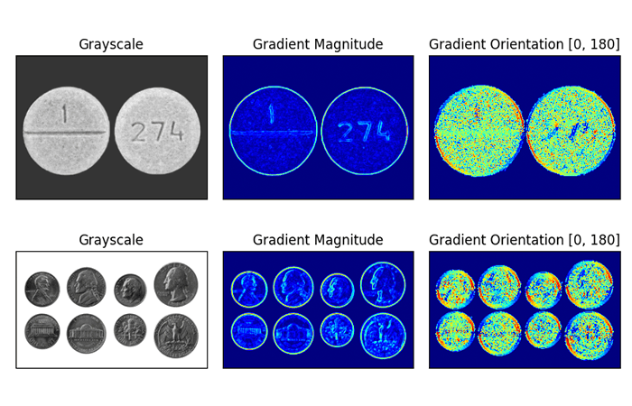
Image gradients are a fundamental building block of many computer vision and image processing routines.

• We use gradients for detecting edges in images, which allows us to find contours and outlines of objects in images
• We use them as inputs for quantifying images through feature extraction — in fact, highly successful and well-known image descriptors such as Histogram of Oriented Gradients and SIFT are built upon image gradient representations
• Gradient images are even used to construct saliency maps, which highlight the subjects of an image

While image gradients are not often discussed in detail since other, more powerful and interesting methods build on top of them, we are going to take the time and discuss them in detail.

To learn how to compute Sobel and Scharr gradients with OpenCV just keep reading.

Image Gradients with OpenCV (Sobel and Scharr)

In the first part of this tutorial, we’ll discuss what image gradients, what they are used for, and how we can compute them manually (that way we have an intuitive understanding).

From there we’ll learn about Sobel and Scharr kernels, which are convolutional filters, allowing us to compute the image gradients automatically using OpenCV and the cv2.Sobel function (we simply pass in a Scharr-specific argument to cv2.Sobel to compute Scharr gradients).

We’ll then configure our development environment and review our project directory structure, where you’ll implement two Python scripts:

1. One to compute the gradient magnitude
2. And another to compute gradient orientation

Together, these computations power traditional computer vision techniques such as SIFT and Histogram of Oriented Gradients.

We’ll wrap up this tutorial with a discussion of our results.

What are image gradients?

As I mentioned in the introduction, image gradients are used as the basic building blocks in many computer vision and image processing applications.

However, the main application of image gradients lies within edge detection.

As the name suggests, edge detection is the process of finding edges in an image, which reveals structural information regarding the objects in an image. Edges could therefore correspond to:

• Boundaries of an object in an image
• Boundaries of shadowing or lighting conditions in an image
• Boundaries of “parts” within an object

Below is an image of edges being detected in an image:

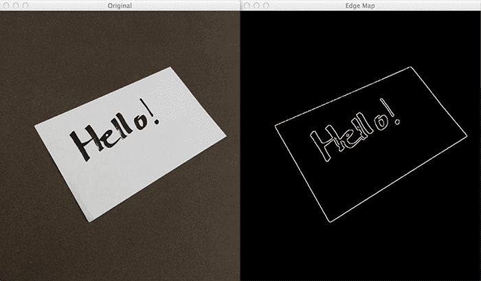
On the left, we have our original input image. On the right, we have our image with detected edges — commonly called an edge map.

The image on the right clearly reveals the structure and outline of the objects in an image. Notice how the outline of the notecard, along with the words written on the notecard, are clearly revealed.

Using this outline, we could then apply contours to extract the actual objects from the region or quantify the shapes so we can identify them later. Just as image gradients are building blocks for methods like edge detection, edge detection is also a building block for developing a complete computer vision application.

Computing image gradients manually

So how do we go about finding these edges in an image?

The first step is to compute the gradient of the image. Formally, an image gradient is defined as a directional change in image intensity.

Or put more simply, at each pixel of the input (grayscale) image, a gradient measures the change in pixel intensity in a given direction. By estimating the direction or orientation along with the magnitude (i.e. how strong the change in direction is), we are able to detect regions of an image that look like edges.

In practice, image gradients are estimated using kernels or filters, just like we did using smoothing and blurring — but this time we are trying to find the structural components of the image. Our goal here is to find the change in direction to the central pixel marked in red in both the x and y direction:

However, before we dive into kernels for gradient estimation, let’s actually go through the process of computing the gradient manually. The first step is to simply find and mark the north, south, east and west pixels surrounding the center pixel:

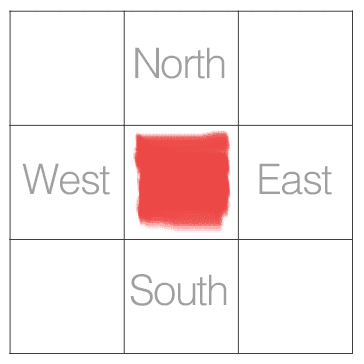
In the image above, we examine the 3×3 neighborhood surrounding the central pixel. Our x values run from left to right, and our y values from top to bottom. In order to compute any changes in direction we’ll need the north, south, east, and west pixels, which are marked on Figure 3.

If we denote our input image as I, then we define the north, south, east, and west pixels using the following notation:

• North:
• South:
• East:
• West:

Again, these four values are critical in computing the changes in image intensity in both the x and y direction.

To demonstrate this, let’s compute the vertical change or the y-change by taking the difference between the south and north pixels:

G_y = I(x, y + 1) – I(x, y − 1)

Similarly, we can compute the horizontal change or the x-change by taking the difference between the east and west pixels:

G_x = I(x + 1, y) – I(x − 1, y)

Awesome — so now we have G_x and G_y, which represent the change in image intensity for the central pixel in both the x and y direction.

So now the big question becomes: what do we do with these values?

To answer that, we’ll need to define two new terms — the gradient magnitude and the gradient orientation.

The gradient magnitude is used to measure how strong the change in image intensity is. The gradient magnitude is a real-valued number that quantifies the “strength” of the change in intensity.

The gradient orientation is used to determine in which direction the change in intensity is pointing. As the name suggests, the gradient orientation will give us an angle or ? that we can use to quantify the direction of the change.

For example, take a look at the following visualization of gradient orientation:

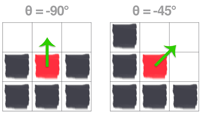
On the left, we have a 3×3 region of an image, where the top half of the image is white and the bottom half of the image is black. The gradient orientation is thus equal to .

And on the right, we have another 3×3 neighborhood of an image, where the upper triangular region is white and the lower triangular region is black. Here we can see the change in direction is equal to .

So I’ll be honest — when I was first introduced to computer vision and image gradients, Figure 4 confused the living hell out of me. I mean, how in the world did we arrive at these calculations of ??! Intuitively, the changes in direction make sense since we can actually see and visualize the result.

But how do we actually go about computing the gradient orientation and magnitude?

I’m glad you asked. Let’s see if we can demystify the gradient orientation and magnitude calculation.

Let’s go ahead and start off with an image of our trusty 3×3 neighborhood of an image:

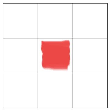
Here, we can see that the central pixel is marked in red. The next step in determining the gradient orientation and magnitude is actually to compute the changes in gradient in both the x and y direction. Luckily, we already know how to do this — they are simply the G_x and G_y values that we computed earlier!

Using both G_x and G_y, we can apply some basic trigonometry to compute the gradient magnitude G, and orientation ?:

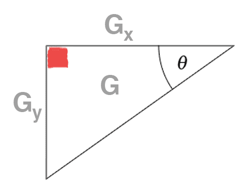
Seeing this example is what really solidified my understanding of gradient orientation and magnitude. Inspecting this triangle you can see that the gradient magnitude G is the hypotenuse of the triangle. Therefore, all we need to do is apply the Pythagorean theorem and we’ll end up with the gradient magnitude:

The gradient orientation can then be given as the ratio of G_y to G_x. Technically we would use the to compute the gradient orientation, but this could lead to undefined values — since we are computer scientists, we’ll use the function to account for the different quadrants instead (if you’re unfamiliar with the arc-tangent, you can read more about it here):

The function gives us the orientation in radians, which we then convert to degrees by multiplying by the ratio of 180/?.

Let’s go ahead and manually compute G and ? so we can see how the process is done:

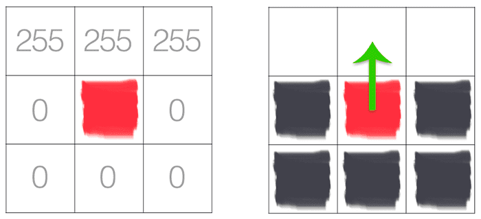
In the above image, we have an image where the upper-third is white and the bottom two-thirds is black. Using the equations for G_x and G_y, we arrive at:

G_x = 0 − 0 = 0

and:

G_y = 0 − 255 = −255

Plugging these values into our gradient magnitude equation we get:

As for our gradient orientation:

See, computing the gradient magnitude and orientation isn’t too bad!

Let’s do another example for fun:

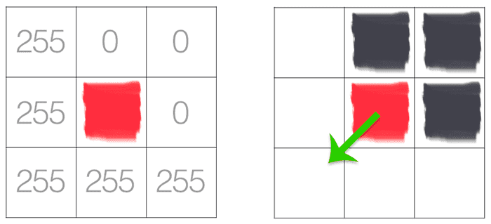
In this particular image, we can see that the lower-triangular region of the neighborhood is white, while the upper-triangular neighborhood is black. Computing both G_x and G_y we arrive at:

G_x = 0 − 255 = −255 and G_y = 255 − 0 = 255

which leaves us with a gradient magnitude of:

and a gradient orientation of:

Sure enough, our gradient is pointing down and to the left at an angle of .

Of course, we have only computed our gradient orientation and magnitude for two unique pixel values: 0 and 255. Normally you would be computing the orientation and magnitude on a grayscale image where the valid range of values would be [0, 255].

Sobel and Scharr Filter

Now that we have learned how to compute gradients manually, let’s look at how we can approximate them using kernels, which will give us a tremendous boost in speed. Just like we used kernels to smooth and blur an image, we can also use kernels to compute our gradients.

We’ll start off with the Sobel method or Sobel filter, which actually uses two kernels/filters: one for detecting horizontal changes in direction and the other for detecting vertical changes in direction:

Given an input image neighborhood below, let’s compute the Sobel approximation to the gradient:

Therefore:

and:

Given these values of G_x and G_y, it would then be trivial to compute the gradient magnitude G and orientation ?:

We could also use the Scharr kernel instead of the Sobel filter which may give us better approximations to the gradient:

The exact reasons as to why the Scharr kernel could lead to better approximations are heavily rooted in mathematical details and are well outside our discussion of image gradients.

If you’re interested in reading more about the Scharr versus Sobel filters and constructing an optimal image gradient approximation (and can read German), I would suggest taking a look at Scharr’s dissertation on the topic.

Overall, gradient magnitude and orientation make for excellent features and image descriptors when quantifying and abstractly representing an image.

But for edge detection, the gradient representation is extremely sensitive to local noise. We’ll need to add in a few more steps to create an actual robust edge detector — we’ll be covering these steps in detail in the next tutorial where we review the Canny edge detector.

Configuring your development environment

To follow this guide, you need to have the OpenCV library installed on your system.

Luckily, OpenCV is pip-installable:

$ pip install opencv-contrib-python

If you need help configuring your development environment for OpenCV, I highly recommend that you read my pip install OpenCV guide — it will have you up and running in a matter of minutes.

Having problems configuring your development environment?

All that said, are you:

• Short on time?
• Learning on your employer’s administratively locked system?
• Wanting to skip the hassle of fighting with the command line, package managers, and virtual environments?
• Ready to run the code right now on your Windows, macOS, or Linux system?

Then join PyImageSearch University today!

Gain access to Jupyter Notebooks for this tutorial and other PyImageSearch guides that are pre-configured to run on Google Colab’s ecosystem right in your web browser! No installation required.

And best of all, these Jupyter Notebooks will run on Windows, macOS, and Linux!

Project structure

Before we implement image gradients with OpenCV, let’s first review our project directory structure.

Be sure to access the “Downloads” section of this tutorial to retrieve the source code and example images:

$ tree . --dirsfirst
.
├── images
│   ├── bricks.png
│   ├── clonazepam_1mg.png
│   ├── coins01.png
│   └── coins02.png
├── opencv_magnitude_orientation.py
└── opencv_sobel_scharr.py

1 directory, 6 files

We will implement two Python scripts today:

1. opencv_sobel_scharr.py: Utilizes the Sobel and Scharr filters to compute gradient information for an input image.
2. opencv_magnitude_orientation.py: Takes the output of a Sobel/Scharr filter and then computes gradient magnitude and orientation information.

The images directory contains various example images that we’ll apply both of these scripts to.

Implementing Scharr and Sobel Filters with OpenCV

Up until this point, we have been discussing a lot of the theory and mathematical details surrounding image kernels. But how do we actually apply what we have learned using OpenCV?

I’m so glad you asked.

Open a new file, name it opencv_sobel_scharr.py, and let’s get coding:

# import the necessary packages
import argparse
import cv2

# construct the argument parser and parse the arguments
ap = argparse.ArgumentParser()
ap.add_argument("-i", "--image", type=str, required=True,
	help="path to input image")
ap.add_argument("-s", "--scharr", type=int, default=0,
	help="path to input image")
args = vars(ap.parse_args())

Lines 2 and 3 import our required Python packages — all we need is argparse for command line arguments and cv2 for our OpenCV bindings.

We then have two command line arguments:

1. --image: The path to our input image residing on disk that we want to compute Sobel/Scharr gradients for.
2. --scharr: Whether or not we are computing Scharr gradients. By default, we’ll compute Soble gradients. If we pass in a value > 0 for this flag then we’ll compute Scharr gradients instead

Let’s now load our image and process it:

# load the image, convert it to grayscale, and display the original
# grayscale image
image = cv2.imread(args["image"])
gray = cv2.cvtColor(image, cv2.COLOR_BGR2GRAY)
cv2.imshow("Gray", gray)

Lines 15-17 load our image from disk, convert it to grayscale (since we compute gradient representations on the grayscale version of the image), and display it on our screen.

# set the kernel size, depending on whether we are using the Sobel
# filter or the Scharr operator, then compute the gradients along
# the x and y axis, respectively
ksize = -1 if args["scharr"] > 0 else 3
gX = cv2.Sobel(gray, ddepth=cv2.CV_32F, dx=1, dy=0, ksize=ksize)
gY = cv2.Sobel(gray, ddepth=cv2.CV_32F, dx=0, dy=1, ksize=ksize)

# the gradient magnitude images are now of the floating point data
# type, so we need to take care to convert them back a to unsigned
# 8-bit integer representation so other OpenCV functions can operate
# on them and visualize them
gX = cv2.convertScaleAbs(gX)
gY = cv2.convertScaleAbs(gY)

# combine the gradient representations into a single image
combined = cv2.addWeighted(gX, 0.5, gY, 0.5, 0)

# show our output images
cv2.imshow("Sobel/Scharr X", gX)
cv2.imshow("Sobel/Scharr Y", gY)
cv2.imshow("Sobel/Scharr Combined", combined)
cv2.waitKey(0)

Computing both the G_x and G_y values is handled on Lines 23 and 24 by making a call to cv2.Sobel. Specifying a value of dx=1 and dy=0 indicates that we want to compute the gradient across the x direction. And supplying a value of dx=0 and dy=1 indicates that we want to compute the gradient across the y direction.

Note: In the event that we want to use the Scharr filter instead of the Sobel filter we simply specify our --scharr command line argument to be > 0 — from there the appropriate ksize is set (Line 22).

However, at this point, both gX and gY are now of the floating point data type. If we want to visualize them on our screen we need to convert them back to 8-bit unsigned integers. Lines 30 and 31 take the absolute value of the gradient images and then squish the values back into the range [0, 255].

Finally, we combine gX and gY into a single image using the cv2.addWeighted function, weighting each gradient representation equally.

Lines 37-40 then show our output images on our screen.

Sobel and Scharr Filter results

Let’s learn how to apply Sobel and Scharr kernels with OpenCV.

Be sure to access the “Downloads” section of this tutorial to retrieve the source code and example images.

From there, open a terminal window and execute the following command:

$ python opencv_sobel_scharr.py --image images/bricks.png

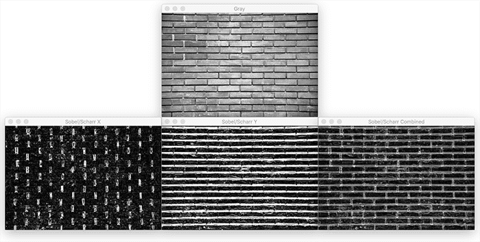
At the top, we have our original image, which is an image of a brick wall.

The bottom-left then displays the Sobel gradient image along the x direction. Notice how computing the Sobel gradient along the x direction reveals the vertical mortar regions of the bricks.

Similarly, the bottom-center shows that Sobel gradient computed along the y direction — now we can see the horizontal mortar regions of the bricks.

Finally, we can add gX and gY together and receive our final output image on the bottom-right.

Let’s look at another image:

$ python opencv_sobel_scharr.py --image images/coins01.png

This time we are investigating a set of coins. Much of the Sobel gradient information is found along the borders/outlines of the coins.

Now, let’s compute the Scharr gradient information for the same image:

$ python opencv_sobel_scharr.py --image images/coins01.png \
	--scharr 1

Notice how the Scharr operator contains more information than the previous example.

Let’s look at another Sobel example:

$ python opencv_sobel_scharr.py --image images/clonazepam_1mg.png

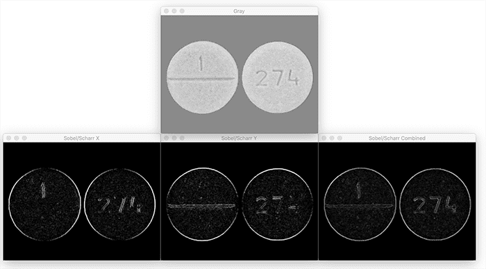
Here, we have computed the Sobel gradient representation of the pill. The outline of the pill is clearly visible, as well as the digits on the pill itself.

Now let’s look at the Scharr representation:

$ python opencv_sobel_scharr.py --image images/clonazepam_1mg.png \
	--scharr 1

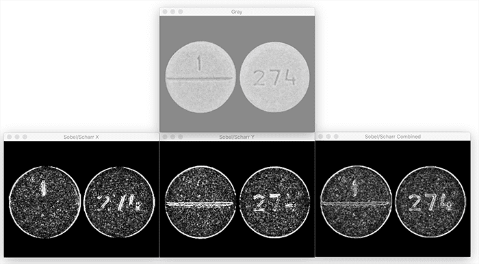
The borders of the pill are just as defined, and what’s more, the Scharr gradient representation is picking up much more of the texture of the pill itself.

Whether or not you use the Sobel or Scharr gradient for your application is dependent on your project, but in general, keep in mind that the Scharr version is going to appear more “visually noisy,” but at the same time captures more nuanced details in the texture.

Computing gradient magnitude and orientation with OpenCV

Up until this point, we’ve learned how to compute the Sobel Filter and Scharr operator, but we don’t have much of an intuition as to what these gradients actually represent.

In this section, we are going to compute the gradient magnitude and gradient orientation of our input grayscale image and visualize the results. Then, in the next section, we’ll review these results, allowing you to obtain a deeper understanding of what gradient magnitude and orientation actually represent.

With that said, open a new file, name it opencv_magnitude_orienation.py, and insert the following code:

# import the necessary packages
import matplotlib.pyplot as plt
import numpy as np
import argparse
import cv2

# construct the argument parser and parse the arguments
ap = argparse.ArgumentParser()
ap.add_argument("-i", "--image", type=str, required=True,
	help="path to input image")
args = vars(ap.parse_args())

Lines 2-5 import our required Python packages, including matplotlib for plotting, NumPy for numerical array processing, argparse for command line arguments, and cv2 for our OpenCV bindings.

We then parse our command line arguments on Lines 8-11. We only need a single switch here, --image, which is the path to our input image residing on disk.

Let’s load our image now and compute the gradient magnitude and orientation:

# load the input image and convert it to grayscale
image = cv2.imread(args["image"])
gray = cv2.cvtColor(image, cv2.COLOR_BGR2GRAY)

# compute gradients along the x and y axis, respectively
gX = cv2.Sobel(gray, cv2.CV_64F, 1, 0)
gY = cv2.Sobel(gray, cv2.CV_64F, 0, 1)

# compute the gradient magnitude and orientation
magnitude = np.sqrt((gX ** 2) + (gY ** 2))
orientation = np.arctan2(gY, gX) * (180 / np.pi) % 180

Lines 14 and 15 load our image from disk and convert it to grayscale.

We then compute the Sobel gradients along the x and y axis, just like we did in the previous section.

However, unlike the previous section, we are not going to display the gradient images to our screen (at least not via the cv2.imshow function), thus we do not have to convert them back into the range [0, 255] or use the cv2.addWeighted function to combine them together.

Instead, we continue with our gradient magnitude and orientation calculations on Lines 22 and 23. Notice how these two lines match our equations above exactly.

The gradient magnitude is simply the square-root of the squared gradients in both the x and y direction added together.

And the gradient orientation is the arc-tangent of the gradients in both the x and y direction.

Let’s now visualize both the gradient magnitude and gradient orientation:

# initialize a figure to display the input grayscale image along with
# the gradient magnitude and orientation representations, respectively
(fig, axs) = plt.subplots(nrows=1, ncols=3, figsize=(8, 4))

# plot each of the images
axs[0].imshow(gray, cmap="gray")
axs[1].imshow(magnitude, cmap="jet")
axs[2].imshow(orientation, cmap="jet")

# set the titles of each axes
axs[0].set_title("Grayscale")
axs[1].set_title("Gradient Magnitude")
axs[2].set_title("Gradient Orientation [0, 180]")

# loop over each of the axes and turn off the x and y ticks
for i in range(0, 3):
	axs[i].get_xaxis().set_ticks([])
	axs[i].get_yaxis().set_ticks([])

# show the plots
plt.tight_layout()
plt.show()

Line 27 creates a figure with one row and three columns (one for the original image, gradient magnitude representation, and one for the gradient orientation representation, respectively).

We then add each of the grayscale, gradient magnitude, and gradient orientation images to the plot (Lines 30-32) while setting the titles for each of the axes (Lines 35-37).

Finally, we turn off axis ticks (Lines 40-42) and display the result on our screen.

Gradient magnitude and orientation results

We are now ready to compute our gradient magnitude!

Start by accessing the “Downloads” section of this tutorial to retrieve the source code and example images.

From there, execute the following command:

$ python opencv_magnitude_orientation.py --image images/coins02.png

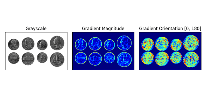
On the left, we have our original input image of coins.

The middle displays the gradient magnitude using the Jet colormap.

Values that are closer to the blue range are very small. For example, the background of the image has a gradient of 0 because there is no gradient there.

Values that are closer to the yellow/red range are quite large (relative to the rest of the values). Taking a look at the outlines/borders of the coins you can see that these pixels have a large gradient magnitude due to the fact that they contain edge information.

Finally, the image on the right displays the gradient orientation information, again using the Jet colormap.

Values here fall into the range [0, 180], where values closer to zero show as blue and values closer to 180 as red. Note that much of the orientation information is contained within the coin itself.

Let’s try another example:

$ python opencv_magnitude_orientation.py \
	--image images/clonazepam_1mg.png

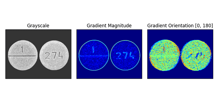
The image on the left contains our input image of a prescription pill meditation. We then compute the gradient magnitude in the middle and display the gradient orientation on the right.

Similar to our coins example, much of the gradient magnitude information lies on the borders/boundaries of the pill while the gradient orientation is much more pronounced due to the texture of the pill itself.

In our next tutorial, you’ll learn how to use this gradient information to detect edges in an input image.

Summary

In this lesson, we defined what an image gradient is: a directional change in image intensity.

We also learned how to manually compute the change in direction surrounding a central pixel using nothing more than the neighborhood of pixel intensity values.

We then used these changes in direction to compute our gradient orientation — the direction in which the change in intensity is pointing — and the gradient magnitude, which is how strong the change in intensity is.

Of course, computing the gradient orientation and magnitude using our simple method is not the fastest way. Instead, we can rely on the Sobel and Scharr Filters, which allow us to obtain an approximation to the image derivative. Similar to smoothing and blurring, our image kernels convolve our input image with a filter that is designed to approximate our gradient.

Finally, we learned how to use the cv2.Sobel OpenCV function to compute Sobel and Scharr gradient representations. Using these gradient representations we were able to pinpoint which pixels in the image had an orientation within the range .

Image gradients are one of the most important image processing and computer vision building blocks you’ll learn about. Behind the scenes, they are used for powerful image descriptor methods such as Histogram of Oriented Gradients and SIFT.

They are used to construct saliency maps to reveal the most “interesting” regions of an image.

And as we’ll see in the next tutorial, we’ll see how image gradients are the cornerstone of the Canny edge detector for detecting edges in images.

Frequently Asked Questions:

To download the source code to this post (and be notified when future tutorials are published here on PyImageSearch), simply enter your email address in the form below!