OpenCV Saliency Detection

Today’s tutorial is on saliency detection, the process of applying image processing and computer vision algorithms to automatically locate the most “salient” regions of an image.

In essence, saliency is what “stands out” in a photo or scene, enabling your eye-brain connection to quickly (and essentially unconsciously) focus on the most important regions.

For example — consider the figure at the top of this blog post where you see a soccer field with players on it. When looking at the photo, your eyes automatically focus on the players themselves as they are the most important areas of the photo. This automatic process of locating the important parts of an image or scene is called saliency detection.

Saliency detection is applied to many aspects of computer vision and image processing, but some of the more popular applications of saliency include:

• Object detection — Instead of exhaustively applying a sliding window and image pyramid, only apply our (computationally expensive) detection algorithm to the most salient, interesting regions of an image most likely to contain an object
• Advertising and marketing — Design logos and ads that “pop” and “stand out” to us from a quick glance
• Robotics — Design robots with visual systems that are similar to our own

In the rest of today’s blog post, you will learn how to perform saliency detection using Python and OpenCV’s saliency module — keep reading to learn more!

OpenCV Saliency Detection with Python

Today’s post was inspired by PyImageSearch Gurus course member, Jeff Nova.

Inside one of the threads in the private PyImageSearch Gurus community forums Jeff wrote:

Great question, Jeff!

And to be totally honest, I had completely forgotten about OpenCV’s saliency module.

Jeff’s question motivated me to do some research on the saliency module in OpenCV. After a few hours of research, trial and error, and just simply playing with the code, I was able to perform saliency detection using OpenCV.

Since there aren’t many tutorials on how to perform saliency detection, especially with the Python bindings, I wanted to write up a tutorial and share it with you.

Enjoy it and I hope it helps you bring saliency detection to your own algorithms.

Three different saliency detection algorithms

In OpenCV’s saliency module there are three primary forms of saliency detection:

1. Static saliency: This class of saliency detection algorithms relies on image features and statistics to localize the most interesting regions of an image.
2. Motion saliency: Algorithms in this class typically rely on video or frame-by-frame inputs. The motion saliency algorithms process the frames, keeping track of objects that “move”. Objects that move are considered salient.
3. Objectness: Saliency detection algorithms that compute “objectness” generate a set of “proposals”, or more simply bounding boxes of where it thinks an object may lie in an image.

Keep in mind that computing saliency is not object detection. The underlying saliency detection algorithm has no idea if there is a particular object in an image or not.

Instead, the saliency detector is simply reporting where it thinks an object may lie in the image — it is up to you and your actual object detection/classification algorithm to:

1. Process the region proposed by the saliency detector
2. Predict/classify the region and make any decisions on this prediction

Saliency detectors are often very fast algorithms capable of running in real-time. The results of the saliency detector are then passed into more computationally expensive algorithms that you would not want to run on every single pixel of the input image.

OpenCV’s saliency detectors

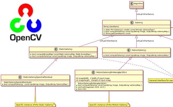
To utilize OpenCV’s saliency detectors you will need OpenCV 3 or greater. OpenCV’s official documentation on their saliency module can be found on this page.

Keep in mind that you will need to have OpenCV compiled with the contrib module enabled. If you have followed any of my OpenCV install tutorials on PyImageSearch you will have the contrib module installed.

Note: I found that OpenCV 3.3 does not work with the motion saliency method (covered later in this blog post) but works with all other saliency implementations. If you find yourself needing motion saliency be sure you are using OpenCV 3.4 or greater.

You can check if the saliency module is installed by opening up a Python shell and trying to import it:

$ python
>>> import cv2
>>> cv2.saliency
<module 'cv2.saliency'>

If the import succeeds, congrats — you have the contrib extra modules installed! But if the import fails, you will need to follow one of my guides to install OpenCV with the contrib modules.

OpenCV provides us with four implementations of saliency detectors with Python bindings, including:

• cv2.saliency.ObjectnessBING_create()
• cv2.saliency.StaticSaliencySpectralResidual_create()
• cv2.saliency.StaticSaliencyFineGrained_create()
• cv2.saliency.MotionSaliencyBinWangApr2014_create()

Each of the above constructors returns an object implementing a .computeSaliency method — we call this method on our input image, returning a two-tuple of:

• A boolean indicating if computing the saliency was successful or not
• The output saliency map which we can use to derive the most “interesting” regions of an image

In the remainder of today’s blog post, I will show you how to perform saliency detection using each of these algorithms.

Saliency detection project structure

Be sure to visit the “Downloads” section of the blog post to grab the Python scripts, image files, and trained model files.

From there, our project structure can be viewed in a terminal using the tree command:

$ tree --dirsfirst
.
├── images
│   ├── barcelona.jpg
│   ├── boat.jpg
│   ├── neymar.jpg
│   └── players.jpg
├── objectness_trained_model [9 entries]
│   ├── ObjNessB2W8HSV.idx.yml.gz
│   ├── ...
├── static_saliency.py
├── objectness_saliency.py
└── motion_saliency.py

2 directories, 16 files

In our project folder we have two directories:

• image/ : A selection of testing images.
• objectness_trained_model/ : This is our model directory for the Objectness Saliency. Included are 9 .yaml files which comprising the objectness model iteslf.

We’re going to review three example scripts today:

• static_saliency.py : This script implements two forms of Static Saliency (based on image features and statistics). We’ll be reviewing this script first.
• objectness_saliency.py : Uses the BING Objectness Saliency method to generate a list of object proposal regions.
• motion_saliency.py : This script will take advantage of your computer’s webcam and process live motion frames in real-time. Salient regions are computed using the Wang and Dudek 2014 method covered later in this guide.

Static saliency

OpenCV implements two algorithms for static saliency detection.

1. The first method is from Montabone and Soto’s 2010 publication, Human detection using a mobile platform and novel features derived from a visual saliency mechanism. This algorithm was initially used for detecting humans in images and video streams but can also be generalized to other forms of saliency as well.
2. The second method is by Hou and Zhang in their 2007 CVPR paper, Saliency detection: A spectral residual approach.

This static saliency detector operates on the log-spectrum of an image, computes saliency residuals in this spectrum, and then maps the corresponding salient locations back to the spatial domain. Be sure to refer to the paper for more details.

Let’s go ahead and try both of these static saliency detectors. Open up static_salency.py and insert the following code:

# import the necessary packages
import argparse
import cv2

# construct the argument parser and parse the arguments
ap = argparse.ArgumentParser()
ap.add_argument("-i", "--image", required=True,
	help="path to input image")
args = vars(ap.parse_args())

# load the input image
image = cv2.imread(args["image"])

On Lines 2 and 3 we import argparse and cv2 . The argparse module will allow us to parse a single command line argument — the --input image (Lines 6-9). OpenCV (with the contrib module) has everything we need to compute static saliency maps.

If you don’t have OpenCV installed you may follow my OpenCV installation guides. At the risk of being a broken record, I’ll repeat my recommendation that you should grab at least OpenCV 3.4 as I had trouble with OpenCV 3.3 for motion saliency further down in this blog post.

We then load the image into memory on Line 12.

Our first static saliency method is static spectral saliency. Let’s go ahead and compute the saliency map of the image and display it:

# initialize OpenCV's static saliency spectral residual detector and
# compute the saliency map
saliency = cv2.saliency.StaticSaliencySpectralResidual_create()
(success, saliencyMap) = saliency.computeSaliency(image)
saliencyMap = (saliencyMap * 255).astype("uint8")
cv2.imshow("Image", image)
cv2.imshow("Output", saliencyMap)
cv2.waitKey(0)

Using the cv2.saliency module and calling the StaticSaliencySpectralResidual_create() method, a static spectral residual saliency object is instantiated (Line 16).

From there we invoke the computeSaliency method on Line 17 while passing in our input image .

What’s the result?

The result is a saliencyMap , a floating point, grayscale image that highlights the most prominent, salient regions of the image. The range of floating point values is [0, 1] with values closer to 1 being the “interesting” areas and values closer to 0 being “uninteresting”.

Are we ready to visualize the output?

Not so fast! Before we can display the map, we need to scale the values to the range [0, 255] on Line 18.

From there, we can display the original image and saliencyMap image to the screen (Lines 19 and 20) until a key is pressed (Line 21).

The second static saliency method we’re going to apply is called “fine grained”. This next block mimics our first method, with the exception that we’re instantiating the fine grained object. We’re also going to perform a threshold to demonstrate a binary map that you might process for contours (i.e., to extract each salient region). Let’s see how it is done:

# initialize OpenCV's static fine grained saliency detector and
# compute the saliency map
saliency = cv2.saliency.StaticSaliencyFineGrained_create()
(success, saliencyMap) = saliency.computeSaliency(image)

# if we would like a *binary* map that we could process for contours,
# compute convex hull's, extract bounding boxes, etc., we can
# additionally threshold the saliency map
threshMap = cv2.threshold(saliencyMap.astype("uint8"), 0, 255,
	cv2.THRESH_BINARY | cv2.THRESH_OTSU)[1]

# show the images
cv2.imshow("Image", image)
cv2.imshow("Output", saliencyMap)
cv2.imshow("Thresh", threshMap)
cv2.waitKey(0)

On Line 25, we instantiate the fine grained static saliency object. From there we compute the saliencyMap on Line 26.

The contributors for this code of OpenCV implemented the fine grained saliency differently than the spectral saliency. This time our values are already scaled in the range [0, 255], so we can go ahead and display on Line 36.

One task you might perform is to compute a binary threshold image so that you can find your likely object region contours. This is performed on Lines 31 and 32 and displayed on Line 37. The next steps would be a series of erosions and dilations (morphological operations) prior to finding and extracting contours. I’ll leave that as an exercise for you.

To execute the static saliency detector be sure to download the source code and example to this post (see the “Downloads” section below) and then execute the following command:

$ python static_saliency.py --image images/neymar.jpg

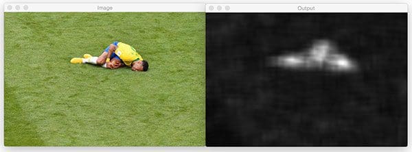
The image of Brazilian professional soccer player, Neymar Jr. first undergoes the spectral method:

And then, after pressing a key, the fine grained method saliency map image is shown. This time I also display a threshold of the saliency map (which easily could have been applied to the spectral method as well):

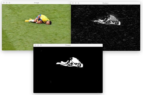
The fine grained map more closely resembles a human than the blurry blob in the previous spectral saliency map. The thresholded image in the bottom center would be a useful starting point in a pipeline to extract the ROI of the likely object.

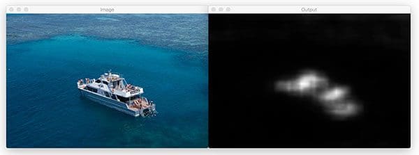
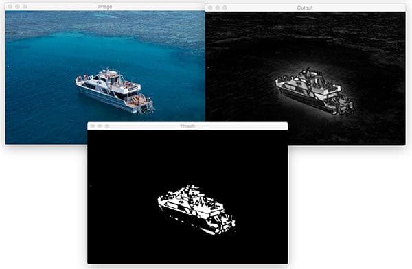
Now let’s try both methods on a photo of a boat:

$ python static_saliency.py --image images/boat.jpg

The static spectral saliency map of the boat:

And fine grained:

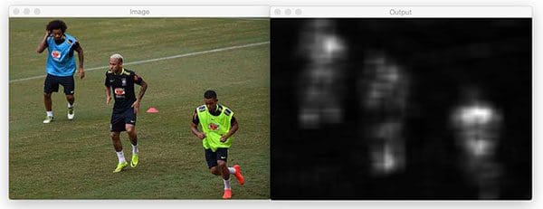
And finally, let’s try both the spectral and fine grained static saliency methods on a picture of three soccer players:

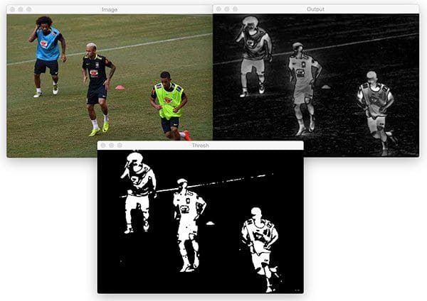
$ python static_saliency.py --image images/players.jpg

Here’s the output of spectral saliency:

As well as fine-grained saliency detection:

Objectness saliency

OpenCV includes one objectness saliency detector — BING: Binarized normed gradients for objectness estimation at 300fps, by Cheng et al. (CVPR 2014).

Unlike the other saliency detectors in OpenCV which are entirely self-contained in their implementation, the BING saliency detector requires nine separate model files for various window sizes, color spaces, and mathematical operations.

The nine model files together are very small (~10KB) and extremely fast, making BING an excellent method for saliency detection.

To see how we can use this objectness saliency detector with OpenCV open up objectness_saliency.py and insert the following code:

# import the necessary packages
import numpy as np
import argparse
import cv2

# construct the argument parser and parse the arguments
ap = argparse.ArgumentParser()
ap.add_argument("-m", "--model", required=True,
	help="path to BING objectness saliency model")
ap.add_argument("-i", "--image", required=True,
	help="path to input image")
ap.add_argument("-n", "--max-detections", type=int, default=10,
	help="maximum # of detections to examine")
args = vars(ap.parse_args())

# load the input image
image = cv2.imread(args["image"])

On Lines 2-4 we import our necessary packages. For this script, we’ll make use of NumPy, argparse , and OpenCV.

From there we parse three command line arguments on Lines 7-14:

• --model : The path to the BING objectness saliency model.
• --image : Our input image path.
• --max-detections : The maximum number of detections to examine with the default set to 10 .

Next, we load our image into memory (Line 17).

Let’s compute objectness saliency:

# initialize OpenCV's objectness saliency detector and set the path
# to the input model files
saliency = cv2.saliency.ObjectnessBING_create()
saliency.setTrainingPath(args["model"])

# compute the bounding box predictions used to indicate saliency
(success, saliencyMap) = saliency.computeSaliency(image)
numDetections = saliencyMap.shape[0]

On Line 21 we initialize the objectness saliency detector followed by establishing the training path on Line 22.

Given these two actions, we can now compute the objectness saliencyMap on Line 25.

The number of available saliency detections can be obtained by examining the shape of the returned NumPy array (Line 26).

Now let’s loop over each of the detections (up to our set maximum):

# loop over the detections
for i in range(0, min(numDetections, args["max_detections"])):
	# extract the bounding box coordinates
	(startX, startY, endX, endY) = saliencyMap[i].flatten()
	
	# randomly generate a color for the object and draw it on the image
	output = image.copy()
	color = np.random.randint(0, 255, size=(3,))
	color = [int(c) for c in color]
	cv2.rectangle(output, (startX, startY), (endX, endY), color, 2)

	# show the output image
	cv2.imshow("Image", output)
	cv2.waitKey(0)

On Line 29, we begin looping over the detections up to the maximum detection count which is contained within our command line args dictionary.

Inside the loop, we first extract the bounding box coordinates (Line 31).

Then we copy the image for display purposes (Line 34), followed by assigning a random color to the bounding box (Lines 35-36).

To see OpenCV’s objectness saliency detector in action be sure to download the source code + example images and then execute the following command:

$ python objectness_saliency.py --model objectness_trained_model 
	--image images/barcelona.jpg

Here you can see that the objectness saliency method does a good job proposing regions of the input image where both Lionel Messi and Luis Saurez are standing/kneeling on the pitch.

You can imagine taking each of these proposed bounding box regions and passing them into a classifier or object detector for further prediction — and best of all, this method would be more computationally efficient than exhaustively applying a series of image pyramids and sliding windows.

Motion saliency

The final OpenCV saliency detector comes from Wang and Dudek’s 2014 publication, A fast self-tuning background subtraction algorithm.

This algorithm is designed to work on video feeds where objects that move in the video feed are considered salient.

Open up motion_saliency.py and insert the following code:

# import the necessary packages
from imutils.video import VideoStream
import imutils
import time
import cv2

# initialize the motion saliency object and start the video stream
saliency = None
vs = VideoStream(src=0).start()
time.sleep(2.0)

We’re going to be working directly with our webcam in this script, so we first import the VideoStream class from imutils on Line 2. We’ll also imutils itself, time , and OpenCV (Lines 3-5).

Now that our imports are out of the way, we’ll initialize our motion saliency object and kick off our threaded VideoStream object (Line 9).

From there we’ll begin looping and capturing a frame at the top of each cycle:

# loop over frames from the video file stream
while True:
	# grab the frame from the threaded video stream and resize it
	# to 500px (to speedup processing)
	frame = vs.read()
	frame = imutils.resize(frame, width=500)

	# if our saliency object is None, we need to instantiate it
	if saliency is None:
		saliency = cv2.saliency.MotionSaliencyBinWangApr2014_create()
		saliency.setImagesize(frame.shape[1], frame.shape[0])
		saliency.init()

On Line 16 we grab a frame followed by resizing it on Line 17. Reducing the size of the frame will allow the image processing and computer vision techniques inside the loop to run faster. The less data there is to process, the faster our pipeline can run.

Lines 20-23 instantiate OpenCV’s motion saliency object if it isn’t already established. For this script we’re using the Wang method, as the constructor is aptly named.

Next, we’ll compute the saliency map and display our results:

	# convert the input frame to grayscale and compute the saliency
	# map based on the motion model
	gray = cv2.cvtColor(frame, cv2.COLOR_BGR2GRAY)
	(success, saliencyMap) = saliency.computeSaliency(gray)
	saliencyMap = (saliencyMap * 255).astype("uint8")

	# display the image to our screen
	cv2.imshow("Frame", frame)
	cv2.imshow("Map", saliencyMap)
	key = cv2.waitKey(1) & 0xFF
 
	# if the `q` key was pressed, break from the loop
	if key == ord("q"):
		break

# do a bit of cleanup
cv2.destroyAllWindows()
vs.stop()

We convert the frame to grayscale (Line 27) and subsequently compute our saliencyMap (Line 28) — the Wang method requires grayscale frames.

As the saliencyMap contains float values in the range [0, 1], we scale to the range [0, 255] and ensure that the value is an unsigned 8-bit integer (Line 29).

From there, we display the original frame and the saliencyMap on Lines 32 and 33.

We then check to see if the quit key (“q”) is pressed, and if it is, we break out of the loop and cleanup (Lines 34-42). Otherwise, we’ll continue to process and display saliency maps to our screen.

To execute the motion saliency script enter the following command:

$ python motion_saliency.py

Below I have recorded an example demo of OpenCV’s motion saliency algorithm in action:

OpenCV Version Note: Motion Saliency didn’t work for me in OpenCV 3.3 (and didn’t throw an error either). I tested in 3.4 and 4.0.0-pre and it worked just fine so make sure you are running OpenCV 3.4 or better if you intend on applying motion saliency.

Summary

In today’s blog post you learned how to perform saliency detection using OpenCV and Python.

In general, saliency detectors fall into three classes of algorithms:

1. Static saliency
2. Motion saliency
3. Objectness saliency

OpenCV provides us with four implementations of saliency detectors with Python bindings, including:

1. cv2.saliency.ObjectnessBING_create()
2. cv2.saliency.StaticSaliencySpectralResidual_create()
3. cv2.saliency.StaticSaliencyFineGrained_create()
4. cv2.saliency.MotionSaliencyBinWangApr2014_create()

I hope this guide helps you apply saliency detection using OpenCV + Python to your own applications!

To download the source code to today’s post (and be notified when future blog posts are published here on PyImageSearch), just enter your email address in the form below!