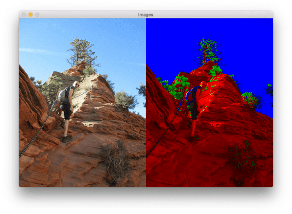
Today’s blog post comes straight out of the PyImageSearch Gurus course. Inside PyImageSearch Gurus we have a community page (much like a combination of forums + Q&A + StackOverflow) where we discuss a variety of computer vision topics, ask questions, and hold each other accountable to learning computer vision and image processing.
This post was inspired by PyImageSearch Gurus member Christian Smith who asked if it was possible to implement GIMP’s Maximum RGB filter using OpenCV and Python:

This thread sparked a great discussion on the topic and even led to an implementation (which I’ll share with you today).
The Max RGB filter isn’t used in many image processing pipelines; however, it’s a very useful tool to use when visualizing the Red, Green, and Blue channels of an image — and which channel contributes most to a given area of an image. It’s also a great filter to use for simple color-based segmentation.
In the remainder of this post I’ll demonstrate how you can implement the Max RGB filter in surprisingly few lines of Python and OpenCV code.
What is the Max RGB filter?
The Max RGB filter is an extremely simple and straight forward image processing filter. The algorithm goes something like this.
- For each pixel in the image I:
- Grab the r, g, and b pixel intensities located at I[x, y]
- Determine the maximum value of r, g, and b: m = max(r, g, b)
- If r < m: r = 0
- If g < m: g = 0
- If b < m: b = 0
- Store the r, g, and b values back in image: I[x, y] = (r, g, b)
The only caveat to mention is if two channels have the same intensity, such as: (155, 98, 155). In this case, both values are kept and the smallest is reduced to zero: (155, 0, 155).
The output image should look something like this:
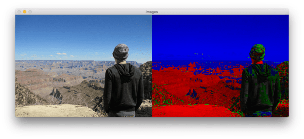
Where we can see the original image on the left and the output filtered image on the right.
Implementing GIMP’s Max RGB filter in OpenCV
Now that we have a good grasp on the Max RGB filter algorithm (and what the intended output is supposed to look like), let’s go ahead and implement it in Python and OpenCV. Open up a new file, name it max_filter.py , and insert the following code:
# import the necessary packages
import numpy as np
import argparse
import cv2

def max_rgb_filter(image):
	# split the image into its BGR components
	(B, G, R) = cv2.split(image)

	# find the maximum pixel intensity values for each
	# (x, y)-coordinate,, then set all pixel values less
	# than M to zero
	M = np.maximum(np.maximum(R, G), B)
	R[R < M] = 0
	G[G < M] = 0
	B[B < M] = 0

	# merge the channels back together and return the image
	return cv2.merge([B, G, R])
Lines 2-4 simply import our necessary packages.
Line 6 defines our max_rgb_filter function. This method requires only a single argument, the image we want to filter.
Given our input image , we then use the cv2.split function to split the image into its respective, Blue, Green, and Red components (Line 8)
Note: It’s important to remember that OpenCV stores images in BGR order rather than RGB. This can cause a bit of a confusion and some hard to track down bugs if you’re just getting started with OpenCV.
Given our R , G , and B channels, we then use NumPy’s maximum method (Line 13) to find the maximum intensity value at each (x, y)-coordinate across all three R , G , and B channels
It’s very important that you use np.maximum and not np.max! The np.max method will only find the maximum value across the entire array as opposed to np.maximum which find the max value at each (x, y)-coordinate.
From there, Lines 14-16 suppress the Red, Green, and Blue pixel intensities that fall below the maximum value M.
Finally, Line 19 merges the channels back together (again, in BGR order since that is what OpenCV expects) and returns the Max RGB filtered image to the calling function.
Now that the max_rgb_filter method is defined, all we need to do is write some code to load our image off disk, apply the Max RGB filter, and display the results to our screen:
# import the necessary packages
import numpy as np
import argparse
import cv2

def max_rgb_filter(image):
	# split the image into its BGR components
	(B, G, R) = cv2.split(image)

	# find the maximum pixel intensity values for each
	# (x, y)-coordinate,, then set all pixel values less
	# than M to zero
	M = np.maximum(np.maximum(R, G), B)
	R[R < M] = 0
	G[G < M] = 0
	B[B < M] = 0

	# merge the channels back together and return the image
	return cv2.merge([B, G, R])

# construct the argument parse and parse the arguments
ap = argparse.ArgumentParser()
ap.add_argument("-i", "--image", required=True,
	help="path to input image")
args = vars(ap.parse_args())

# load the image, apply the max RGB filter, and show the
# output images
image = cv2.imread(args["image"])
filtered = max_rgb_filter(image)
cv2.imshow("Images", np.hstack([image, filtered]))
cv2.waitKey(0)
This code should be fairly self-explanatory. Lines 22-25 handle parsing our command line arguments. The only switch we need is --image , the path to where the image we want to process resides on disk.
From there, Lines 29-32 handle loading our image , applying the Max RGB filter, and finally displaying both the original and filtered image to our screen.
To see our script in action, just open up your terminal and execute the following command:
$ python max_filter.py --image images/horseshoe_bend_02.jpg
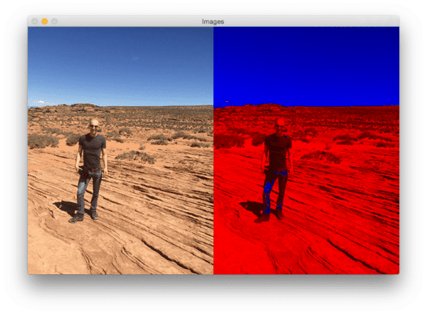
On the left we have the original image — a photo of myself in the desert near Horseshoe Bend, AZ. Then, on the right we have the image after our Max RGB filter has been applied. At the top of the image we can see the sky is a rich blue, indicating that the blue channel has larger pixel intensity values in that region. Opposite the blue sky, the bottom of the image is more red (they don’t call it redstone for nothin’) — here the red channel has large pixel intensity values and the green and blue channel are suppressed.
Let’s give another image a try:
$ python max_filter.py --image images/max_filter_horseshoe_bend_01.png
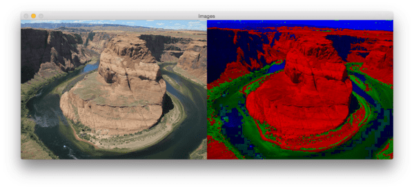
I especially like this image since it highlights how water is not always a “clear blue” like we think it is. Not surprisingly, the redstone is highlighted in red and the sky is very much blue. However, the water itself is a mixture of both blue and green. Furthermore, both these regions of water are clearly segmented from each other.
Let’s do one final example:
$ python max_filter.py --image images/max_filter_antelope_canyon.png
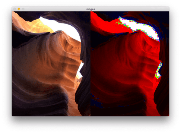
This image is from Antelope Canyon in Page, AZ (probably one of the most beautiful areas in the world). At the bottom of the slot canyon there is very little light so we don’t see much color at all (although if we you look closely you can see patches of deep blue/purple which the caverns are known for). Then, as we move our way up the canyon walls more light is let in, revealing the wonderful red glow. Finally, at the top of the cavern is the sky which is so bright in this photo it’s washed out.
Like I said, it’s rare that we use the Max RGB filter in image processing pipelines; however, since the filter allows you to investigate which channels of an image contribute most to a given region, it’s a valuable tool to have when performing basic segmentation and debugging.
What's next? We recommend PyImageSearch University.
86+ total classes • 115+ hours hours of on-demand code walkthrough videos • Last updated: May 2026
★★★★★ 4.84 (128 Ratings) • 16,000+ Students Enrolled
I strongly believe that if you had the right teacher you could master computer vision and deep learning.
Do you think learning computer vision and deep learning has to be time-consuming, overwhelming, and complicated? Or has to involve complex mathematics and equations? Or requires a degree in computer science?
That’s not the case.
All you need to master computer vision and deep learning is for someone to explain things to you in simple, intuitive terms. And that’s exactly what I do. My mission is to change education and how complex Artificial Intelligence topics are taught.
If you're serious about learning computer vision, your next stop should be PyImageSearch University, the most comprehensive computer vision, deep learning, and OpenCV course online today. Here you’ll learn how to successfully and confidently apply computer vision to your work, research, and projects. Join me in computer vision mastery.
Inside PyImageSearch University you'll find:
- ✓ 86+ courses on essential computer vision, deep learning, and OpenCV topics
- ✓ 86 Certificates of Completion
- ✓ 115+ hours hours of on-demand video
- ✓ Brand new courses released regularly, ensuring you can keep up with state-of-the-art techniques
- ✓ Pre-configured Jupyter Notebooks in Google Colab
- ✓ Run all code examples in your web browser — works on Windows, macOS, and Linux (no dev environment configuration required!)
- ✓ Access to centralized code repos for all 540+ tutorials on PyImageSearch
- ✓ Easy one-click downloads for code, datasets, pre-trained models, etc.
- ✓ Access on mobile, laptop, desktop, etc.
Summary
Today’s blog post was inspired by a question asked by Christian Smith, a member of PyImageSearch Gurus (thanks Christian!). Christian asked if it was possible to implement GIMP’s Max RGB filter using nothing but Python and OpenCV — obviously, the answer is yes. But what may be surprisingly is how few lines of code it can be done in!
Go ahead and download the code to this post and apply the Max RGB filter to your own images. See if you can guess which Red, Green, or Blue channel contributes most to a specific region of an image — you might be surprised how your intuition and perception of color is wrong in certain circumstances!
Finally, if you’re interested in joining the PyImageSearch Gurus course, please be sure to click here and claim your spot in line. Spots inside the course are limited (only small batches of readers are let in at a time), so it’s very important that your claim your spot if you’re interested in the course!

Download the Source Code and FREE 17-page Resource Guide
Enter your email address below to get a .zip of the code and a FREE 17-page Resource Guide on Computer Vision, OpenCV, and Deep Learning. Inside you'll find my hand-picked tutorials, books, courses, and libraries to help you master CV and DL!
