Build DeepSeek-V3: Multi-Head Latent Attention (MLA) Architecture

---

---

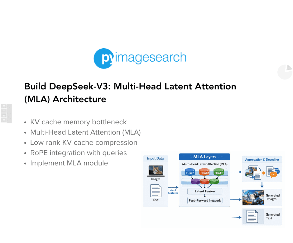
Build DeepSeek-V3: Multi-Head Latent Attention (MLA) Architecture

In the first part of this series, we laid the foundation by exploring the theoretical underpinnings of DeepSeek-V3 and implementing key configuration elements such as Rotary Positional Embeddings (RoPE). That tutorial established how DeepSeek-V3 manages long-range dependencies and sets up its architecture for efficient scaling. By grounding theory in working code, we ensured that readers not only understood the concepts but also saw how they translate into practical implementation.

With that groundwork in place, we now turn to one of DeepSeek-V3’s most distinctive innovations: Multi-Head Latent Attention (MLA). While traditional attention mechanisms have proven remarkably effective, they often come with steep computational and memory costs. MLA reimagines this core operation by introducing a latent representation space that dramatically reduces overhead while preserving the model’s ability to capture rich contextual relationships.

In this lesson, we’ll break down the theory behind MLA, explore why it matters, and then implement it step by step. This installment continues our hands-on approach — moving beyond abstract concepts to practical code — while advancing the broader goal of the series: to reconstruct DeepSeek-V3 from scratch, piece by piece, until we assemble and train the full architecture.

This lesson is the 2nd of the 6-part series on Building DeepSeek-V3 from Scratch:

1. DeepSeek-V3 Model: Theory, Config, and Rotary Positional Embeddings
2. Build DeepSeek-V3: Multi-Head Latent Attention (MLA) Architecture (this tutorial)
3. Lesson 3
4. Lesson 4
5. Lesson 5
6. Lesson 6

To learn about DeepSeek-V3 and build it from scratch, just keep reading.

---

The KV Cache Memory Problem in DeepSeek-V3

To understand why MLA is revolutionary, we must first understand the memory bottleneck in Transformer inference. Standard multi-head attention computes:

,

where are query, key, and value matrices for sequence length . In autoregressive generation (producing one token at a time), we cannot recompute attention over all previous tokens from scratch at each step — that would be computation per token generated.

Instead, we cache the key and value matrices. When generating token , we only compute (the query for the new token), then compute attention using and the cached . This reduces computation from to per generated token — a dramatic speedup.

However, this cache comes at a steep memory cost. For a model with layers, attention heads, and head dimension , the KV cache requires:

.

For a model like GPT-3 with 96 layers, 96 heads, 128-head dimensions, and 2048 sequence length, this is:

.

This means you can only serve a handful of users concurrently on even high-end GPUs. The memory bottleneck is often the limiting factor in deployment, not computation.

---

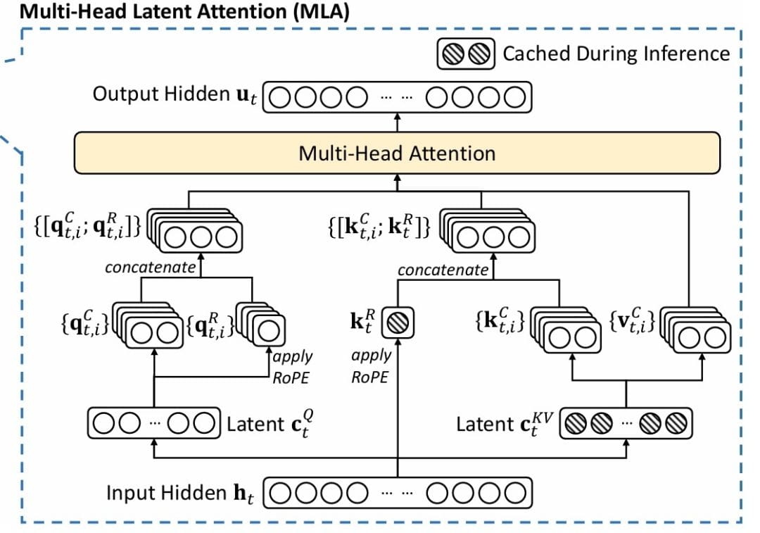
Multi-Head Latent Attention (MLA): KV Cache Compression with Low-Rank Projections

MLA (Figure 1) solves this through a compress-decompress strategy inspired by Low-Rank Adaptation (LoRA). The key insight: we do not need to store full -dimensional representations. We can compress them into a lower-dimensional latent space for storage, then decompress when needed for computation.

Step 1. Key-Value Compression: Instead of storing directly, we project them through a low-rank bottleneck:

,

where is the input, is the down-projection, and is the low-rank dimension. We only cache rather than the full and .

Step 2. Key-Value Decompression: When we need the actual key and value matrices for attention computation, we decompress:

,

where are up-projection matrices. This decomposition approximates the full key and value matrices through a low-rank factorization: and .

Memory Savings: Instead of caching , we cache . The reduction factor is . For our configuration with and , this is a 4× reduction. For larger models with and , it’s a 16× reduction — transformative for deployment.

---

Query Compression and Rotary Positional Embeddings (RoPE) Integration

MLA extends compression to queries, though less aggressively since queries are not cached:

,

where can be different from . In our configuration, versus — we give queries slightly more capacity.

Now comes the clever part: integrating RoPE. We split both queries and keys into content and positional components:

,

where denotes concatenation. The content components come from the compression-decompression process described above. The positional components are separate projections that we apply RoPE to:

,

where denotes applying rotary embedding at position . This separation is crucial: content and position are independently represented and combined only in the attention scores.

---

Attention Computation with Multi-Head Latent Attention (MLA)

The complete attention computation becomes:

.

Then standard multi-head attention:

,

where are per-head projections. The attention scores naturally incorporate both content similarity (through ) and positional information (through ).

Causal Masking: For autoregressive language modeling, we must prevent tokens from attending to future positions. We apply a causal mask:

.

This ensures position can only attend to positions , maintaining the autoregressive property.

Attention Weights and Output: After computing scores with the causal mask applied:

,

where is the effective key dimension (content plus RoPE dimensions). We apply attention to values:

,

where is the output projection. Finally, dropout is applied for regularization, and the result is added to the residual connection.

---

Implementation: Multi-Head Latent Attention (MLA)

Here is the complete implementation of MLA:

class MultiheadLatentAttention(nn.Module):
    """
    Multihead Latent Attention (MLA) - DeepSeek's efficient attention mechanism

    Key innovations:
    - Compression/decompression of queries and key-values
    - LoRA-style low-rank projections for efficiency
    - RoPE with separate content and positional components
    """

    def __init__(self, config: DeepSeekConfig):
        super().__init__()
        self.config = config
        self.n_embd = config.n_embd
        self.n_head = config.n_head
        self.head_dim = config.n_embd // config.n_head

        # Compression dimensions
        self.kv_lora_rank = config.kv_lora_rank
        self.q_lora_rank = config.q_lora_rank
        self.rope_dim = config.rope_dim

Lines 11-21: Configuration and Dimensions. We extract key parameters from the configuration object, computing the head dimension as . We store compression ranks (kv_lora_rank and q_lora_rank) and the RoPE dimension. These define the memory-accuracy tradeoff — lower ranks mean more compression but potentially lower quality. Our choices balance efficiency with model capacity.

        # KV decompression
        self.k_decompress = nn.Linear(self.kv_lora_rank, self.n_head * self.head_dim, bias=False)
        self.v_decompress = nn.Linear(self.kv_lora_rank, self.n_head * self.head_dim, bias=False)

        # Query compression
        self.q_proj = nn.Linear(self.n_embd, self.q_lora_rank, bias=False)
        self.q_decompress = nn.Linear(self.q_lora_rank, self.n_head * self.head_dim, bias=False)

        # RoPE projections
        self.k_rope_proj = nn.Linear(self.n_embd, self.n_head * self.rope_dim, bias=False)
        self.q_rope_proj = nn.Linear(self.q_lora_rank, self.n_head * self.rope_dim, bias=False)

        # Output projection
        self.o_proj = nn.Linear(self.n_head * self.head_dim, self.n_embd, bias=config.bias)

        # Dropout
        self.attn_dropout = nn.Dropout(config.dropout)
        self.resid_dropout = nn.Dropout(config.dropout)

        # RoPE
        self.rope = RotaryEmbedding(self.rope_dim, config.block_size)

        # Causal mask
        self.register_buffer(
            "causal_mask",
            torch.tril(torch.ones(config.block_size, config.block_size)).view(
                1, 1, config.block_size, config.block_size
            )
        )

Lines 23-29: KV Compression Pipeline. The compression-decompression architecture follows the low-rank factorization principle. The kv_proj layer performs the down-projection from to , cutting the dimensionality in half. We apply RMSNorm to the compressed representation for stability — this normalization helps prevent the compressed representation from drifting to extreme values during training. The decompression layers k_decompress and v_decompress then expand back to dimensions. Note that we use bias=False for these projections — empirical research shows that biases in attention projections do not significantly help and add unnecessary parameters.

Lines 31-33: Query Processing and RoPE Projections. Query handling follows a similar compression pattern but with a slightly higher rank (). The asymmetry makes sense: we do not cache queries, so memory pressure is lower, and we can afford more capacity. The RoPE projections are separate pathways — k_rope_proj projects directly from the input , while q_rope_proj projects from the compressed query representation. Both target the RoPE dimension of 64. This separation of content and position is architecturally elegant: the model learns different transformations for “what” (content) versus “where” (position).

Lines 36-51: Infrastructure Components. The output projection o_proj combines multi-head outputs back to the model dimension. We include 2 dropout layers:

• attn_dropout: applied to attention weights (reducing overfitting on attention patterns)
• resid_dropout: applied to the final output (regularizing the residual connection)

The RoPE module is instantiated with our chosen dimension and maximum sequence length. Finally, we create and register a causal mask as a buffer — by using register_buffer, this tensor moves with the model to GPU/CPU and is included in the state dict, but is not treated as a learnable parameter.

    def forward(self, x: torch.Tensor, attention_mask: Optional[torch.Tensor] = None):
        B, T, C = x.size()

        # Compression phase
        kv_compressed = self.kv_norm(self.kv_proj(x))
        q_compressed = self.q_proj(x)

        # Decompression phase
        k_content = self.k_decompress(kv_compressed)
        v = self.v_decompress(kv_compressed)
        q_content = self.q_decompress(q_compressed)

        # RoPE components
        k_rope = self.k_rope_proj(x)
        q_rope = self.q_rope_proj(q_compressed)

        # Reshape [B, H, T, d_head] for multi-head attention
        k_content = k_content.view(B, T, self.n_head, self.head_dim).transpose(1, 2)
        v = v.view(B, T, self.n_head, self.head_dim).transpose(1, 2)
        q_content = q_content.view(B, T, self.n_head, self.head_dim).transpose(1, 2)
        k_rope = k_rope.view(B, T, self.n_head, self.rope_dim).transpose(1, 2)
        q_rope = q_rope.view(B, T, self.n_head, self.rope_dim).transpose(1, 2)

        # Apply RoPE
        cos, sin = self.rope(x, T)
        q_rope = apply_rope(q_rope, cos, sin)
        k_rope = apply_rope(k_rope, cos, sin)

        # Concatenate content and rope parts
        q = torch.cat([q_content, q_rope], dim=-1)
        k = torch.cat([k_content, k_rope], dim=-1)

Lines 52-57: Compression Phase. The forward pass begins by compressing the input. We project onto the KV latent space, apply normalization, and project back onto the query latent space. These operations are lightweight — just matrix multiplications. The compressed representations are what we would cache during inference. Notice that kv_compressed has shape versus the original — we’ve already halved the memory footprint.

Lines 60-73: Decompression and RoPE. We decompress to get content components and compute separate RoPE projections. Then comes a crucial reshaping step: we convert from to , moving the head dimension before the sequence dimension. This layout is required for multi-head attention — each head operates independently, and we want to batch those operations. The .transpose(1, 2) operation efficiently swaps dimensions without copying data.

Lines 76-82: RoPE Application and Concatenation. We fetch cosine and sine tensors from our RoPE module and apply the rotation to both queries and keys. Critically, we only rotate the RoPE components, not the content components. This maintains the separation between “what” and “where” information. We then concatenate along the feature dimension, creating final query and key tensors of shape . The attention scores will capture both content similarity and relative position.

        # Attention computation
        scale = 1.0 / math.sqrt(q.size(-1))
        scores = torch.matmul(q, k.transpose(-2, -1)) * scale

        # Apply causal mask
        scores = scores.masked_fill(self.causal_mask[:, :, :T, :T] == 0, float('-inf'))

        # Apply padding mask if provided
        if attention_mask is not None:
            padding_mask_additive = (1 - attention_mask).unsqueeze(1).unsqueeze(2) * float('-inf')
            scores = scores + padding_mask_additive

        # Softmax and dropout
        attn_weights = F.softmax(scores, dim=-1)
        attn_weights = self.attn_dropout(attn_weights)

        # Apply attention to values
        out = torch.matmul(attn_weights, v)

        # Reshape and project
        out = out.transpose(1, 2).contiguous().view(B, T, self.n_head * self.head_dim)
        out = self.resid_dropout(self.o_proj(out))

        return out

Lines 84-94: Attention Score Computation and Masking. We compute scaled dot-product attention: . The scaling factor is critical for training stability — without it, attention logits would grow large as dimensions increase, leading to vanishing gradients in the softmax. We apply the causal mask using masked_fill, setting future positions to negative infinity so they contribute zero probability after softmax. If an attention mask is provided (for handling padding), we convert it to an additive mask and add it to scores. This handles variable-length sequences in a batch.

Lines 97-107: Attention Weights and Output. We apply softmax to convert scores to probabilities, ensuring they sum to 1 over the sequence dimension. Dropout is applied to attention weights — this has been shown to help with generalization, perhaps by preventing the model from becoming overly dependent on specific attention patterns. We multiply attention weights by values to get our output. The final transpose and reshape convert from the multi-head layout back to , concatenating all heads. The output projection and residual dropout complete the attention module.

---

Multi-Head Latent Attention and KV Cache Optimization

Multi-Head Latent Attention (MLA) is one approach to KV cache optimization — compression through low-rank projections. Other approaches include the following:

• Multi-Query Attention (MQA), where all heads share a single key and value
• Grouped-Query Attention (GQA), where heads are grouped to share KV pairs
• KV Cache Quantization, which stores keys and values at lower precision (INT8 or INT4)
• Cache Eviction Strategies, which discard less important past tokens

Each approach has the following trade-offs:

• MQA and GQA reduce quality more than MLA but are simpler
• Quantization can degrade accuracy
• Cache eviction strategies discard historical context

DeepSeek-V3’s MLA offers an appealing middle ground — significant memory savings with minimal quality loss through a principled compression approach.

For readers interested in diving deeper into KV cache optimization, we recommend exploring the “KV Cache Optimization” series, which covers these techniques in detail, including implementation strategies, benchmarking results, and guidance on choosing the right approach for a given use case.

With MLA implemented, we have addressed one of the primary memory bottlenecks in Transformer inference — the KV cache. Our attention mechanism can now serve longer contexts and more concurrent users within the same hardware budget. In the next lesson, we will address another critical challenge: scaling model capacity efficiently through Mixture of Experts (MoE).

---

---

Summary

In this 2nd lesson of our DeepSeek-V3 from Scratch series, we dive into the mechanics of Multi-Head Latent Attention (MLA) and why it is a crucial innovation for scaling large language models.

We begin by introducing MLA and framing it against the KV cache memory problem, a common bottleneck in Transformer architectures. By understanding this challenge, we set the stage for how MLA provides a more efficient solution through compression and smarter attention computation.

We then explore how low-rank projections enable MLA to compress key-value representations without losing essential information. This compression is paired with query compression and RoPE integration, ensuring that positional encoding remains geometrically consistent while reducing computational overhead.

Together, these techniques rethink the attention mechanism, balancing efficiency and accuracy and making MLA a powerful tool for modern architectures.

Finally, we walk through the implementation of MLA, showing how it connects directly to KV cache optimization.

By the end of this lesson, we not only understand the theory but also gain hands-on experience implementing MLA and integrating it into DeepSeek-V3. This practical approach shows how MLA reshapes attention computation, paving the way for more memory-efficient and scalable models.

---

Citation Information

Mangla, P. “Build DeepSeek-V3: Multi-Head Latent Attention (MLA) Architecture,” PyImageSearch, S. Huot, A. Sharma, and P. Thakur, eds., 2026, https://pyimg.co/scgjl

@incollection{Mangla_2026_build-deepseek-v3-mla-architecture,
  author = {Puneet Mangla},
  title = {{Build DeepSeek-V3: Multi-Head Latent Attention (MLA) Architecture}},
  booktitle = {PyImageSearch},
  editor = {Susan Huot and Aditya Sharma and Piyush Thakur},
  year = {2026},
  url = {https://pyimg.co/scgjl},
}

---

To download the source code to this post (and be notified when future tutorials are published here on PyImageSearch), simply enter your email address in the form below!