Table of Contents
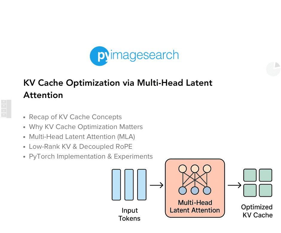
KV Cache Optimization via Multi-Head Latent Attention
Transformer-based language models have long relied on Key-Value (KV) caching to accelerate autoregressive inference. By storing previously computed key and value tensors, models avoid redundant computation across decoding steps. However, as sequence lengths grow and model sizes scale, the memory footprint and compute cost of KV caches become increasingly prohibitive — especially in deployment scenarios that demand low latency and high throughput.
Recent innovations, such as Multi-head Latent Attention (MLA), notably explored in DeepSeek-V2, offer a compelling alternative. Instead of caching full-resolution KV tensors for each attention head, MLA compresses them into a shared latent space using low-rank projections. This not only reduces memory usage but also enables more efficient attention computation without sacrificing model quality.
Inspired by this paradigm, this post dives into the mechanics of KV cache optimization through MLA, unpacking its core components: low-rank KV projection, up-projection for decoding, and a novel twist on rotary position embeddings (RoPE) that decouples positional encoding from head-specific KV storage.
By the end, you’ll see how these techniques converge to form a leaner, faster attention mechanism — one that preserves expressivity while dramatically improving inference efficiency.
This lesson is the 2nd of a 3-part series on LLM Inference Optimization 101 — KV Cache:
- Introduction to KV Cache Optimization Using Grouped Query Attention
- KV Cache Optimization via Multi-Head Latent Attention (this tutorial)
- KV Cache Optimization via Tensor Product Attention
To learn how to optimize KV Cache using Multi-Head Latent Attention, just keep reading.
Recap of KV Cache
Transformers, especially in large language models (LLMs), have become the dominant paradigm for sequence modeling in language, vision, and multimodal AI. At the heart of scalable inference in such models lies the Key-Value (KV) cache, a mechanism central to efficient autoregressive decoding.
As transformers generate text (or other sequences) one token at a time, the attention mechanism computes, caches, and then reuses key (K) and value (V) vectors for all previously seen tokens in the sequence. This enables the model to avoid redundant recomputation, reducing both the computational time and energy required to generate each new token.
Technically, for an input sequence of length  , at each layer and for each attention head, the model produces queries
  , keys
  , and values
  . In classic Multi-Head Attention (MHA), the computation for a single attention head is:
 = \text{softmax}\left(\dfrac{Q K^\top}{\sqrt{d_k}}\right) V,")
where  is the dimension of the key and query vectors per head. The need to attend to all previous tokens for every new token pushes computational complexity from
 ") (without caching) to
(without caching) to ") (with caching), where
(with caching), where  is sequence length.
During autoregressive inference, caching is crucial. For each new token, the previously computed K and V vectors from all prior tokens are stored and reused; new K/V for the just-generated token are added to the cache. The process can be summarized in a simple workflow:
- For the first token, compute and cache K/V
- When generating further tokens:
- Compute Q for the current token
- Retrieve all cached K/V
- Compute attention using current Q and cached K/V
- Update the cache with the new K/V
Despite its simple elegance in enabling linear-time decoding, the KV cache quickly becomes a bottleneck in large-scale, long-context models. Its memory usage scales as:
 \times \text{Layers} \times \text{Precision}")
This can easily reach dozens of gigabytes for high-end LLMs, often dwarfing the space needed just for model weights. For instance, in Llama-2-7B with a context window of 28,000 tokens, KV cache use is comparable to model weights — about 14 GB in FP16.
A direct result is that inference performance is no longer bounded solely by compute — it becomes bound by memory bandwidth and capacity. On current GPUs, the bottleneck shifts from floating-point ops to reading and writing very wide matrices as the token context expands. Autoregressive generation, already a sequential (non-parallel) process, gets further constrained.
The Need for KV Cache Optimization
To keep up with LLMs deployed for real-world dialogue, code assistants, and document summarization — often requiring context lengths of 32K tokens and beyond — an efficient KV cache is indispensable. Modern software frameworks such as Hugging Face Transformers, NVIDIA’s FasterTransformer, and vLLM support various cache implementations and quantization strategies to optimize this crucial component.
However, as context windows increase, simply quantizing or sub-sampling cache entries proves insufficient; the redundancy in the hidden dimension of K/V remains untapped, leaving further optimization potential on the table.
This is where Multi-Head Latent Attention (MLA) steps in — it optimizes KV cache storage and memory bandwidth via intelligent, mathematically sound low-rank and latent space projections, enabling transformers to operate efficiently in long-context, high-throughput settings.
Multi-Head Latent Attention (MLA)
Low-Rank KV Projection
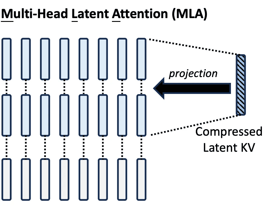
The heart of MLA’s efficiency lies in low-rank projection, a technique that reduces the dimensionality of K/V tensors before caching. Rather than storing full-resolution K/V vectors for each head and each token, MLA compresses them into a shared latent space, leveraging the underlying linear redundancy of natural language and the overparameterization of transformer blocks (Figure 1).
Mathematical Foundations
In standard MHA, for input sequence  and
and  heads, Q, K, V are projected as:

where  is the head dimension. Autoregressive inference makes it necessary to cache K and V for all past steps, leading to a large cache matrix of shape
 ") per layer and per type (K/V).
per layer and per type (K/V).
MLA innovates by introducing latent down-projection matrices:

where 
Here, the model projects Q, K, and V into lower-dimensional latent spaces, where  are significantly smaller than the original dimensions.
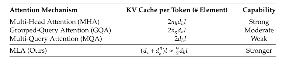
In practice, for a 4096-dimensional model with 32 heads, each with 128 dimensions per head, the standard KV cache requires 4096 values per token per type. MLA reduces this to (e.g., 512 values per token), delivering an 8x reduction in cache size (Table 1).
Up-Projection
After compressing K and V into a shared, low-dimensional latent space, MLA must reconstruct (“up-project”) the full K and V representations when needed for attention computations. This on-demand up-projection is what allows the model to reap storage and bandwidth savings, yet retain high representational and modeling capacity.
Once the sequence has been projected into latent spaces ( for K and V,
  for Q):

where:
 and
and  are low-dimensional latent representations,
 are decompression matrices.
 and
and  are low-dimensional latent representations,
 are decompression matrices.
When computing the attention score:
V = \text{softmax}\left( \dfrac{C_Q W^{Q_{\text{up}},i} \left({W^{K_{\text{up}},i}}\right)^\top}{\sqrt{d_k}}\right)C_{KV} W^{V_\text{up},i}")
where:
- Down-projection: Compresses
 to
to  ,
,  ,
, - Up-projection: Reprojects the latent space to head dimensions via the decompression/up-projection matrices.
 to
to  ,
,Importantly, the multiplication ^\top") is independent of the input and can be precomputed, further saving attention computation at inference.
is independent of the input and can be precomputed, further saving attention computation at inference.
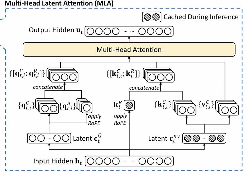
This optimizes both storage (cache only latent vectors) and compute (precompute and cache up-projection weights) (Figure 2).
Decoupled Rotary Position Embeddings (RoPE)
Position information is the crucial ingredient for transformer attention to respect the order of sequences, whether tokens in text or patches in images. Early transformers used absolute or relative position encodings, but these often fell short for long-range or extrapolative contexts.
Rotary Position Embedding (RoPE) is the modern solution, used in leading LLMs (LLAMA, Qwen, Gemma, etc.), leveraging a mathematical trick: position is encoded as a phase rotation in each even-odd pair of embedding dimensions, so the dot product between query and key captures relative position as the angular difference — elegant, parameter-free, and future-proof for long contexts.
RoPE in Standard MHA
Formally, for token position  and embedding index
  :
:
}, x^{(2i+1)} \right)\ = \left( \begin{bmatrix} \cos(\theta_{p,i}) & -\sin(\theta_{p,i}) \\ \sin(\theta_{p,i}) & \cos(\theta_{p,i}) \end{bmatrix} \begin{bmatrix} x^{(2i)} \\ x^{(2i+1)} \end{bmatrix} \right)") with
with ")
determined analytically for each pair and position.
This rotation ensures that the relative position (i.e., the distance between tokens) drives the similarity in attention, enabling powerful extrapolation for long-context and relative reasoning.
Challenges in MLA: The Need for Decoupling
In MLA, the challenge is that the low-rank compression and up-projection pipeline cannot “commute” past the nonlinear rotational operation inherent to RoPE. That is, simply projecting K/V into a latent space and reconstructing later is incompatible with applying the rotation in the standard way post-compression.
To address this, Decoupled RoPE is introduced:
- Split the key and query representations into positional and non-positional (NoPE) components before compression
- Apply RoPE only to the positional portions (typically a subset of the head dimensions)
- Leave the bulk of the compressed, latent representations unrotated
- Concatenate these before final attention score computation
Mathematically, for head  :
:
} = (c_i W_{kc}^{(s)}) \oplus (x_i W_{kr} \mathcal{R}_i)")
where  is concatenation,
  is the low-rank latent vector,
 }") is head-specific up-projection,
is head-specific up-projection,  is projection to the RoPE subspace, and
  is the rotation matrix at position .
Queries are treated analogously. This split enables MLA’s memory efficiency while preserving RoPE’s powerful relative position encoding.
PyTorch Implementation of Multi-Head Latent Attention
In this section, we will see how using Multi-head Latent Attention improves the KV Cache size. For simplicity, we will implement a toy transformer model with 1 layer of RoPE-less Multi-Head Latent Attention.
Multi-Head Latent Attention
We will start by implementing the Multi-head Latent Attention in PyTorch. For simplicity, we will use a RoPE-less variant of Multi-head Latent Attention in this implementation.
import torch
import torch.nn as nn
import time
import matplotlib.pyplot as plt
import math

class MultiHeadLatentAttention(nn.Module):
    def __init__(self, d_model=4096, num_heads=128, q_latent_dim=12, kv_latent_dim=4):
        super().__init__()
        self.d_model = d_model
        self.num_heads = num_heads
        self.q_latent_dim = q_latent_dim
        self.kv_latent_dim = kv_latent_dim
        head_dim = d_model // num_heads

        # Query projections
        self.Wq_d = nn.Linear(d_model, q_latent_dim)

        # Precomputed matrix multiplications of W_q^U and W_k^U, for multiple heads
        self.W_qk = nn.Linear(q_latent_dim, num_heads * kv_latent_dim)

        # Key/Value latent projections
        self.Wkv_d = nn.Linear(d_model, kv_latent_dim)
        self.Wv_u = nn.Linear(kv_latent_dim, num_heads * head_dim)

        # Output projection
        self.Wo = nn.Linear(num_heads * head_dim, d_model)

    def forward(self, x, kv_cache):
        batch_size, seq_len, d_model = x.shape

        # Projections of input into latent spaces
        C_q = self.Wq_d(x)     # shape: (batch_size, seq_len, q_latent_dim)
        C_kv = self.Wkv_d(x)   # shape: (batch_size, seq_len, kv_latent_dim)

        # Append to cache
        kv_cache['kv'] = torch.cat([kv_cache['kv'], C_kv], dim=1)

        # Expand KV heads to match query heads
        C_kv = kv_cache['kv']
        # print(C_kv.shape)

        # Attention score, shape: (batch_size, num_heads, seq_len, seq_len)
        C_qW_qk = self.W_qk(C_q).view(batch_size, seq_len, self.num_heads, self.kv_latent_dim)
        scores = torch.matmul(C_qW_qk.transpose(1, 2), C_kv.transpose(-2, -1)[:, None, ...]) / math.sqrt(self.kv_latent_dim)

        # Attention computation
        attn_weight = torch.softmax(scores, dim=-1)
        # Restore V from latent space
        V = self.Wv_u(C_kv).view(batch_size, C_kv.shape[1], self.num_heads, -1)
        # Compute attention output, shape: (batch_size, seq_len, num_heads, head_dim)
        output = torch.matmul(attn_weight, V.transpose(1,2)).transpose(1,2).contiguous()
        # Concatentate the heads, then apply output projection
        output = self.Wo(output.view(batch_size, seq_len, -1))
        return output, kv_cache
This implementation defines a custom PyTorch module for Multi-head Latent Attention (MLA), a memory-efficient variant of standard multi-head attention. On Lines 1-5, we import the necessary libraries, including PyTorch and matplotlib for potential visualization. The class MultiHeadLatentAttention begins on Line 7, where we initialize key hyperparameters: the model dimension d_model, number of heads, and latent dimensions for queries (q_latent_dim) and keys/values (kv_latent_dim).
Notably, d_model is set to 4096, suggesting a high-dimensional input space. On Lines 17-27, we define the projection layers: Wq_d maps input to a low-dimensional query latent space, W_qk transforms queries into head-specific key projections, Wkv_d compresses input into latent KV representations, and Wv_u restores values from latent space for attention output. The final layer Wo projects concatenated attention outputs back to the model dimension.
In the forward method starting on Line 29, we process the input tensor x and a running kv_cache. On Lines 30-34, we project the input into query (C_q) and KV (C_kv) latent spaces. The KV cache is updated on Line 37 by appending the new latent KV representations. On Lines 44 and 45, we compute attention scores by projecting queries into head-specific key spaces (C_qW_qk) and performing scaled dot-product attention against the cached latent keys. This yields a score tensor of shape (batch_size, num_heads, seq_len, seq_len).
On Line 48, we apply softmax to get attention weights and up-project the cached latent values (C_kv) into full-resolution per-head value tensors (V). The final output is computed via a weighted sum of values, reshaped, and passed through the output projection layer on Lines 50-54.
Toy Transformer and Inference
Now that we have implemented the multi-head latent attention module, we will implement a 1-layer toy Transformer block that takes a sequence of input tokens, along with KV Cache, and performs a single feedforward pass.
class TransformerBlock(nn.Module):
    def __init__(self,  d_model=128*128, num_heads=128, q_latent_dim=12, kv_latent_dim=4):
        super().__init__()
        self.attn = MultiHeadLatentAttention(d_model, num_heads, q_latent_dim, kv_latent_dim)
        self.norm1 = nn.LayerNorm(d_model)
        self.ff = nn.Sequential(
            nn.Linear(d_model, d_model * 4),
            nn.ReLU(),
            nn.Linear(d_model * 4, d_model)
        )
        self.norm2 = nn.LayerNorm(d_model)

    def forward(self, x, kv_cache):
        attn_out, kv_cache = self.attn(x, kv_cache)
        x = self.norm1(x + attn_out)
        ff_out = self.ff(x)
        x = self.norm2(x + ff_out)
        return x, kv_cache
We define a TransformerBlock class on Lines 1-11, where the constructor wires together a MultiHead Latent Attention layer (self.attn), two LayerNorms (self.norm1 and self.norm2), and a two-layer feed-forward network (self.ff) that expands the hidden dimension by 4× and then projects it back.
On Lines 13-18, the forward method takes input x and the kv_cache, runs x through the attention module to get attn_out and an updated cache, then applies a residual connection plus layer norm (x = norm1(x + attn_out)). Next, we feed this through the FFN, add another residual connection, normalize again (x = norm2(x + ff_out)), and finally return the transformed hidden states alongside the refreshed kv_cache.
Next, the code snippet below runs an inference to generate a sequence of tokens in an autoregressive manner.
def run_inference(block):
    d_model = block.attn.d_model
    num_heads = block.attn.num_heads
    kv_latent_dim = block.attn.kv_latent_dim

    seq_lengths = list(range(1, 101, 10))
    kv_cache_sizes = []
    inference_times = []

    kv_cache = {
        'kv': torch.empty(1, 0, kv_latent_dim)
    }

    for seq_len in seq_lengths:
        x = torch.randn(1, 1, d_model)  # One token at a time
        start = time.time()
        o, kv_cache = block(x, kv_cache)
        end = time.time()
        # print(o.shape)
        size = kv_cache['kv'].numel()
        kv_cache_sizes.append(size)
        inference_times.append(end - start)

    return seq_lengths, kv_cache_sizes, inference_times
On Lines 1-8, we define run_inference, pull out d_model, num_heads, and kv_latent_dim, and build a list of target seq_lengths (1 to 101 in steps of 10), along with empty lists for kv_cache_sizes and inference_times. On Lines 10-12, we initialize kv_cache with empty tensors for 'kv' of shape [1, 0, kv_latent_dim] so it can grow as we generate tokens.
Then, in the loop over each seq_len on Lines 14-18, we simulate feeding one random token x at a time into the transformer block, timing the forward pass, and updating kv_cache. Finally, on Lines 20-24, we measure the total number of elements in the cached keys and values, append that to kv_cache_sizes, record the elapsed time to inference_times, and at the end return all three lists for plotting or analysis.
Experiments and Analysis
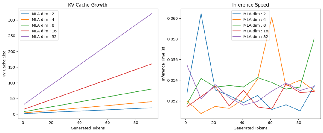
Finally, we will test our implementation of multi-head latent attention with different KV latent dimensions. For each latent dimension, we will plot the size of the KV Cache and inference time as a function of sequence length.
plt.figure(figsize=(12, 5))
plt.subplot(1, 2, 1)

for latent_dim in [2, 4, 8, 16, 32]:
  mla_block = TransformerBlock(d_model=4096, q_latent_dim=12, kv_latent_dim=latent_dim)
  seq_lengths, sizes, times = run_inference(mla_block)
  plt.plot(seq_lengths, sizes, label="MLA dim : {}".format(latent_dim))

plt.xlabel("Generated Tokens")
plt.ylabel("KV Cache Size")
plt.title("KV Cache Growth")
plt.legend()

plt.subplot(1, 2, 2)
for latent_dim in [2, 4, 8, 16, 32]:
    mla_block = TransformerBlock(d_model=4096, q_latent_dim=12, kv_latent_dim=latent_dim)
    seq_lengths, sizes, times = run_inference(mla_block)
    plt.plot(seq_lengths, times, label="MLA dim : {}".format(latent_dim))


plt.xlabel("Generated Tokens")
plt.ylabel("Inference Time (s)")
plt.title("Inference Speed")

plt.legend()

plt.tight_layout()
plt.show()
On Lines 1 and 2, we set up a 12×5-inch figure and declare the first subplot for KV cache growth. Between Lines 4-8, we loop over various latent_dim values, instantiate a TransformerBlock for each, call run_inference to gather sequence lengths and cache sizes, and plot KV cache size versus generated tokens.
On Lines 14-18, we switch to the second subplot, repeat the loop to collect and plot inference times against token counts, and finally, on Lines 21-28, we set axis labels, add a title and legend, tighten the layout, and call plt.show() to render both charts (Figure 3).
What's next? We recommend PyImageSearch University.

120+ total classes • 115+ hours hours of on-demand code walkthrough videos • Last updated: July 2026
★★★★★ 4.84 (128 Ratings) • 16,000+ Students Enrolled
I strongly believe that if you had the right teacher you could master computer vision and deep learning.
Do you think learning computer vision and deep learning has to be time-consuming, overwhelming, and complicated? Or has to involve complex mathematics and equations? Or requires a degree in computer science?
That’s not the case.
All you need to master computer vision and deep learning is for someone to explain things to you in simple, intuitive terms. And that’s exactly what I do. My mission is to change education and how complex Artificial Intelligence topics are taught.
If you're serious about learning computer vision, your next stop should be PyImageSearch University, the most comprehensive computer vision, deep learning, and OpenCV course online today. Here you’ll learn how to successfully and confidently apply computer vision to your work, research, and projects. Join me in computer vision mastery.
Inside PyImageSearch University you'll find:
- ✓ 120+ courses on essential computer vision, deep learning, and OpenCV topics
- ✓ 94+ Certificates of Completion
- ✓ 115+ hours hours of on-demand video
- ✓ Brand new courses released regularly, ensuring you can keep up with state-of-the-art techniques
- ✓ Pre-configured Jupyter Notebooks in Google Colab
- ✓ Run all code examples in your web browser — works on Windows, macOS, and Linux (no dev environment configuration required!)
- ✓ Access to centralized code repos for all 540+ tutorials on PyImageSearch
- ✓ Easy one-click downloads for code, datasets, pre-trained models, etc.
- ✓ Access on mobile, laptop, desktop, etc.
Summary
In this blog post, we explore how Multi-head Latent Attention (MLA) offers a powerful solution to the growing inefficiencies of KV caching in transformer models. We begin by recapping the role of KV caches in autoregressive decoding and highlighting the memory and compute bottlenecks that arise as sequence lengths and model sizes scale. This sets the stage for MLA — a technique that compresses key-value tensors into shared latent spaces, dramatically reducing cache size while preserving attention fidelity. Inspired by DeepSeek’s success, we unpack the architectural motivations and practical benefits of this approach.
We then dive into the core components of MLA: low-rank KV projection, up-projection for decoding, and a novel treatment of rotary position embeddings (RoPE). Through mathematical formulations and intuitive explanations, we show how latent compression and decoupled positional encoding work together to streamline attention computation. The post includes a full PyTorch implementation of MLA, followed by a toy transformer setup to benchmark inference speed and memory usage. By the end, we demonstrate how MLA not only improves efficiency but also opens new doors for scalable, deployable transformer architectures.
Citation Information
Mangla, P. “KV Cache Optimization via Multi-Head Latent Attention,” PyImageSearch, P. Chugh, S. Huot, A. Sharma, and P. Thakur, eds., 2025, https://pyimg.co/bxvc0
@incollection{Mangla_2025_kv-cache-optimization-via-multi-head-latent-attention,
  author = {Puneet Mangla},
  title = {{KV Cache Optimization via Multi-Head Latent Attention}},
  booktitle = {PyImageSearch},
  editor = {Puneet Chugh and Susan Huot and Aditya Sharma and Piyush Thakur},
  year = {2025},
  url = {https://pyimg.co/bxvc0},
}
To download the source code to this post (and be notified when future tutorials are published here on PyImageSearch), simply enter your email address in the form below!

Download the Source Code and FREE 17-page Resource Guide
Enter your email address below to get a .zip of the code and a FREE 17-page Resource Guide on Computer Vision, OpenCV, and Deep Learning. Inside you'll find my hand-picked tutorials, books, courses, and libraries to help you master CV and DL!

Comment section
Hey, Adrian Rosebrock here, author and creator of PyImageSearch. While I love hearing from readers, a couple years ago I made the tough decision to no longer offer 1:1 help over blog post comments.
At the time I was receiving 200+ emails per day and another 100+ blog post comments. I simply did not have the time to moderate and respond to them all, and the sheer volume of requests was taking a toll on me.
Instead, my goal is to do the most good for the computer vision, deep learning, and OpenCV community at large by focusing my time on authoring high-quality blog posts, tutorials, and books/courses.
If you need help learning computer vision and deep learning, I suggest you refer to my full catalog of books and courses — they have helped tens of thousands of developers, students, and researchers just like yourself learn Computer Vision, Deep Learning, and OpenCV.
Click here to browse my full catalog.