Introduction to Distributed Training in PyTorch

In this tutorial, you will learn the basics of distributed training with PyTorch.

This is the last lesson in a 3-part tutorial on intermediate PyTorch techniques for computer vision and deep learning practitioners:

• Image Data Loaders in PyTorch (1st lesson)
• PyTorch: Transfer Learning and Image Classification (last week’s tutorial)
• Introduction to Distributed Training in PyTorch (today’s lesson)

When I first learned about PyTorch, I was quite indifferent to it. As someone who used TensorFlow throughout his Deep Learning days, I wasn’t yet ready to leave the comfort zone TensorFlow had created and try out something new.

As fate would have it, due to some unavoidable circumstances, I had to finally dive into PyTorch. Although to be very honest, I had a rough start. Having been accustomed to hiding behind TensorFlow’s abstractions, the verbose nature of PyTorch reminded me exactly why I had left Java and opted for Python.

However, after a while, the beauty of PyTorch started to unravel itself. The reason why it is more verbose is that it lets you have more control over your actions. Granting you a more definite grasp over every step you take, PyTorch gives you more freedom. Perhaps Java also had the same intention, but I’ll never know since that ship has sailed!

Distributed training presents you with several ways to utilize every bit of computation power you have and make your model training much more efficient. One of PyTorch’s stellar features is its support for Distributed training.

Today, we will learn about the Data Parallel package, which enables a single machine, multi-GPU parallelism. After completing this tutorial, the readers will have:

• A clear understanding of PyTorch’s Data Parallelism
• An idea on implementing Data Parallelism
• A clear vision of your goal while traversing through PyTorch’s verbose code

To learn how to use Data Parallel Training in PyTorch, just keep reading.

Introduction to Distributed Training in PyTorch

What is PyTorch’s Data Parallel training?

Imagine having a computer with 4 RTX 2060 GPUs. You have been given a task where you have to deal with several gigabytes of data. Piece of cake, right? What if you had no way of using all that computation power together? That would be extremely frustrating, almost like if we had a billion dollars but were only allowed to spend $5 a month!

It wouldn’t be ideal if we had no way of using all our resources together. Thankfully, PyTorch has our back! Figure 1 shows how PyTorch utilizes multiple GPUs in a single system in a simple yet efficient manner.

This is known as Data Parallel training, where you are using a single host system with multiple GPUs to boost your efficiency while dealing with huge piles of data.

The Process is as simple as it can be. Once nn.DataParallel is called, individual model instances are created on each of your GPUs. The data is then batched into equal parts, one for each model instance. Finally, each instance creates its own gradients, which are then averaged and back-propagated amongst all the available instances.

Without further ado, let’s jump into the code and see distributed training in action!

Configuring your development environment

To follow this guide, first and foremost, you need to have PyTorch installed in your system. To access PyTorch’s own set of models for vision computing, you will also need to have Torchvision in your system. We are also using the imutils package for data handling. Finally, we will be using matplotlib to plot our results!

Luckily, all of the above-mentioned packages are pip-installable!

$ pip install torch
$ pip install torchvision
$ pip install imutils
$ pip install matplotlib

Having problems configuring your development environment?

All that said, are you:

• Short on time?
• Learning on your employer’s administratively locked system?
• Wanting to skip the hassle of fighting with the command line, package managers, and virtual environments?
• Ready to run the code right now on your Windows, macOS, or Linux system?

Then join PyImageSearch University today!

Gain access to Jupyter Notebooks for this tutorial and other PyImageSearch guides that are pre-configured to run on Google Colab’s ecosystem right in your web browser! No installation required.

And best of all, these Jupyter Notebooks will run on Windows, macOS, and Linux!

Project structure

Before hopping into the project, let’s review the project structure.

$ tree -d .
.
├── distributed_inference.py
├── output
│   ├── food_classifier.pth
│   └── model_training.png
├── prepare_dataset.py
├── pyimagesearch
│   ├── config.py
│   ├── create_dataloaders.py
│   └── food_classifier.py
├── results.png
└── train_distributed.py

2 directories, 9 files

First and foremost, comes the pyimagesearch directory. It houses:

• config.py: houses several important parameters and paths which are used throughout the project
• create_dataloaders.py: houses a function that will help us load, process, and handle datasets
• food_classifier.py: the main model architecture residing inside this script

The other scripts we’ll use are in the parent directory. They are:

• train_distributed.py: defines data processes and trains our model
• distributed_inference.py: will be used to assess our trained model on individual test data

Finally, we have our output folder, which will house all the results (plots, models) that all the other scripts produce.

Configuring the Prerequisites

To begin our implementation, let’s start with config.py, the script that will house the configuration of the end-to-end training and inference pipeline. These values will be used throughout the project.

# import the necessary packages
import torch
import os
 
# define path to the original dataset
DATA_PATH = "Food-11"
 
# define base path to store our modified dataset
BASE_PATH = "dataset"
 
# define paths to separate train, validation, and test splits
TRAIN = os.path.join(BASE_PATH, "training")
VAL = os.path.join(BASE_PATH, "validation")
TEST = os.path.join(BASE_PATH, "evaluation") 

We define a path to our original dataset (Line 6) and a base path (Line 9) to store our modified dataset. On Lines 12-14, we define separate train, validation, and test paths for our modified dataset using the os.path.join function.

# initialize the list of class label names
CLASSES = ["Bread", "Dairy_product", "Dessert", "Egg", "Fried_food",
    "Meat", "Noodles/Pasta", "Rice", "Seafood", "Soup",
    "Vegetable/Fruit"]
 
# specify ImageNet mean and standard deviation and image size
MEAN = [0.485, 0.456, 0.406]
STD = [0.229, 0.224, 0.225]
IMAGE_SIZE = 224

On Lines 17-19, we define our target classes. We are choosing 11 classes into which our dataset will be grouped. On Lines 22-24, we specify the mean, standard deviation, and image size values for our ImageNet input. Notice how the mean and standard deviation have 3 values each. Each value represents the channel-wise, height-wise, and width-wise mean and standard deviation, respectively. The image size is set to 224 × 224 to match the accepted generalized input size of the ImageNet model.

# set the device to be used for training and evaluation
DEVICE = torch.device("cuda")
 
# specify training hyperparameters
LOCAL_BATCH_SIZE = 128
PRED_BATCH_SIZE = 4
EPOCHS = 20
LR = 0.0001
 
# define paths to store training plot and trained model
PLOT_PATH = os.path.join("output", "model_training.png")
MODEL_PATH = os.path.join("output", "food_classifier.pth")

Since today’s task involves demonstrating multiple Graphics Processing Units for training, we will set torch.device to cuda (Line 27). cuda is an ingenious application programming interface (API) developed by NVIDIA, enabling GPUs that are CUDA (Compute Unified Device Architecture) allowed to be used for general purpose processing. Furthermore, since GPUs have more bandwidth and cores than CPUs, they are faster at training machine learning models.

On Lines 30-33, we set up a few hyperparameters like LOCAL_BATCH_SIZE (batch size during training), PRED_BATCH_SIZE (for batch size during inference), epochs, and learning rate. Then, on Lines 36 and 37, we define paths to store our training plot and trained model. The former will assess how well it fared against model metrics, while the latter will be called to the inference module.

For our next task, we’ll move into the create_dataloaders.py script.

# import the necessary packages
from . import config
from torch.utils.data import DataLoader
from torchvision import datasets
import os

def get_dataloader(rootDir, transforms, bs, shuffle=True):
	# create a dataset and use it to create a data loader
	ds = datasets.ImageFolder(root=rootDir,
		transform=transforms)
	loader = DataLoader(ds, batch_size=bs, shuffle=shuffle,
		num_workers=os.cpu_count(),
		pin_memory=True if config.DEVICE == "cuda" else False)

	# return a tuple of the dataset and the data loader
	return (ds, loader)

On Line 7, we define a function called get_dataloader which takes the root directory, PyTorch’s transform instance, and batch size as external arguments.

On Lines 9 and 10, we are using torchvision.datasets.ImageFolder to map all items in the given directory to have the __getitem__ and __len__ methods. These methods have a very important role to play here.

Firstly, they help represent the dataset in a map-like structure from indices to data samples.

Secondly, the newly mapped dataset can now be passed through a torch.utils.data.DataLoader instance (Lines 11-13), which can load multiple data samples in parallel.

Finally, we are returning the dataset and the DataLoader instance (Line 16).

Preparing the Dataset for Distributed Training

For today’s tutorial, we are using the Food-11 dataset. If you’d like a quick way to download the Food-11 Dataset, please refer to this excellent blog post by Adrian on fine-tuning models created using Keras!

Although the dataset already has a training, testing, and validation split, we will organize it in a more easy-to-understand way.

In its original form, the dataset is in a format shown in Figure 3:

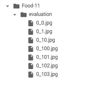
Each filename is in the format class_index_imageNumber.jpg. For example, the file 0_10.jpg refers to an image belonging to the Bread label. Images from all classes are grouped together. In our custom dataset, we will arrange images by their labels and put them in their respective folder with label names. So, after the data preparation, our dataset structure will look something like Figure 4:

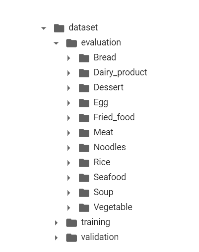
Each label-wise folder will contain respective images belonging to these labels. This is done because many modern frameworks and functions prefer a folder structure like this when processing input.

So, let’s jump into our prepare_dataset.py script and code it out!

# USAGE
# python prepare_dataset.py

# import the necessary packages
from pyimagesearch import config
from imutils import paths
import shutil
import os

def copy_images(rootDir, destiDir):
	# get a list of the all the images present in the directory
	imagePaths = list(paths.list_images(rootDir))
	print(f"[INFO] total images found: {len(imagePaths)}...")

We start by defining a function copy_images (Line 10) which takes two arguments: The root directory where our images are and the destination directory where our custom dataset will be copied. Then, on Line 12, we use the paths.list_images function to generate a list of all images in the root directory. This will be used later while copying the files.

      # loop over the image paths
	for imagePath in imagePaths:
		# extract class label from the filename
		filename = imagePath.split(os.path.sep)[-1]
		label = config.CLASSES[int(filename.split("_")[0])].strip()

		# construct the path to the output directory
		dirPath = os.path.sep.join([destiDir, label])

		# if the output directory does not exist, create it
		if not os.path.exists(dirPath):
			os.makedirs(dirPath)

		# construct the path to the output image file and copy it
		p = os.path.sep.join([dirPath, filename])
		shutil.copy2(imagePath, p)

We start iterating over the list of images on Line 16. First, we single out the exact name of the file by separating the preceding pathname (Line 18), and then we identify the label of the file by filename.split("_")[0]) and feed it to config.CLASSES as an index. In the first pass of the loop, the function creates the directory path (Lines 25 and 26). Finally, we construct the path to the current image and use the shutil package to copy the image to the destination path.

	# calculate the total number of images in the destination
	# directory and print it
	currentTotal = list(paths.list_images(destiDir))
	print(f"[INFO] total images copied to {destiDir}: "
		f"{len(currentTotal)}...")

# copy over the images to their respective directories
print("[INFO] copying images...")
copy_images(os.path.join(config.DATA_PATH, "training"), config.TRAIN)
copy_images(os.path.join(config.DATA_PATH, "validation"), config.VAL)
copy_images(os.path.join(config.DATA_PATH, "evaluation"), config.TEST)

We run a sanity check on Lines 34 and 35 to see if all the files have been copied. This concludes the copy_images function. We call the function on Lines 40-42 and create our modified Train, Test, and Validation dataset!

Creating the PyTorch Classifier

Since our dataset creation is complete, it’s time for us to hop into the food_classifier.py script and define our classifier.

# import the necessary packages
from torch.cuda.amp import autocast
from torch import nn

class FoodClassifier(nn.Module):
	def __init__(self, baseModel, numClasses):
		super(FoodClassifier, self).__init__()

		# initialize the base model and the classification layer
		self.baseModel = baseModel
		self.classifier = nn.Linear(baseModel.classifier.in_features,
			numClasses)

		# set the classifier of our base model to produce outputs
		# from the last convolution block
		self.baseModel.classifier = nn.Identity()

We first define our custom nn.Module class (Line 5). This is normally done when the architecture is more complex, allowing more flexibility while defining our model. Inside the class, our first job is to define the __init__ function to initialize the object’s state.

The super method on Line 7 will enable access to the methods of the base class. Then, on Line 10, we initialize the base model as the baseModel argument that was passed in the constructor (__init__). We then create a separate classification output layer (Line 11) with 11 outputs, each representing one of the classes that we had defined earlier. Finally, since we are using our own classification layer, we replace the inbuilt classifier layer of the baseModel with nn.Identity, which is nothing but a placeholder layer. Hence, the inbuilt classifier of the baseModel will just mirror the outputs of the convolution block just before its classification layer.

	# we decorate the *forward()* method with *autocast()* to enable 
	# mixed-precision training in a distributed manner
	@autocast()
	def forward(self, x):
		# pass the inputs through the base model and then obtain the
		# classifier outputs
		features = self.baseModel(x)
		logits = self.classifier(features)

		# return the classifier outputs
		return logits

On Line 21, we define the forward() pass of our custom model, but before that, we decorate the model with @autocast(). This decorator function enables mixed-precision during training, which essentially makes your training faster due to the smart assignment of data types. I have linked to a blog by TensorFlow, which explains mixed precision in detail. Finally, on Lines 24 and 25, we get the baseModel output and pass it through the custom classifier layer to get the final output.

Using Distributed Training to Train the PyTorch Classifier

Our next destination is the train_distributed.py, where we will put our model training into motion and learn about putting multiple GPUs to use!

# USAGE
# python train_distributed.py

# import the necessary packages
from pyimagesearch.food_classifier import FoodClassifier
from pyimagesearch import config
from pyimagesearch import create_dataloaders
from sklearn.metrics import classification_report
from torchvision.models import densenet121
from torchvision import transforms
from tqdm import tqdm
from torch import nn
from torch import optim
import matplotlib.pyplot as plt
import numpy as np
import torch
import time

# determine the number of GPUs we have
NUM_GPU = torch.cuda.device_count()
print(f"[INFO] number of GPUs found: {NUM_GPU}...")

# determine the batch size based on the number of GPUs
BATCH_SIZE = config.LOCAL_BATCH_SIZE * NUM_GPU
print(f"[INFO] using a batch size of {BATCH_SIZE}...")

The torch.cuda.device_count() function (Line 20) will list the number of CUDA compatible GPUs present in our system. This will be used to determine our global batch size (Line 24), which is config.LOCAL_BATCH_SIZE * NUM_GPU. This is because if our global batch size is B, and we have N CUDA compatible GPUs, each GPU will deal with data of batch size B/N. For example, for a global batch size of 12 and 2 CUDA compatible GPUs, each GPU will assess data of batch size 6.

# define augmentation pipelines
trainTansform = transforms.Compose([
	transforms.RandomResizedCrop(config.IMAGE_SIZE),
	transforms.RandomHorizontalFlip(),
	transforms.RandomRotation(90),
	transforms.ToTensor(),
	transforms.Normalize(mean=config.MEAN, std=config.STD)
])
testTransform = transforms.Compose([
	transforms.Resize((config.IMAGE_SIZE, config.IMAGE_SIZE)),
	transforms.ToTensor(),
	transforms.Normalize(mean=config.MEAN, std=config.STD)
])

# create data loaders
(trainDS, trainLoader) = create_dataloaders.get_dataloader(config.TRAIN,
	transforms=trainTansform, bs=BATCH_SIZE)
(valDS, valLoader) = create_dataloaders.get_dataloader(config.VAL,
	transforms=testTransform, bs=BATCH_SIZE, shuffle=False)
(testDS, testLoader) = create_dataloaders.get_dataloader(config.TEST,
	transforms=testTransform, bs=BATCH_SIZE, shuffle=False)

Next, we use a very handy function by PyTorch, known as torchvision.transforms. Not only does it help build complex transformation pipelines, but it also grants us a lot of control over the transforms we choose to use.

Notice on Lines 28-34, we use several data augmentations for our training set images, like RandomHorizontalFlip, RandomRotation, etc. We also add the mean and standard deviation normalization values to our dataset using this function.

We again use torchvision.transforms for the test transformations (Lines 35-39), but we don’t add additional augmentations. Instead, we pass these instances through the get_dataloader function that we had created in the create_dataloaders script and get the training, validation, and testing datasets and data loaders, respectively (Lines 42-47).

# load up the DenseNet121 model
baseModel = densenet121(pretrained=True)

# loop over the modules of the model and if the module is batch norm,
# set it to non-trainable
for module, param in zip(baseModel.modules(), baseModel.parameters()):
	if isinstance(module, nn.BatchNorm2d):
		param.requires_grad = False

# initialize our custom model and flash it to the current device
model = FoodClassifier(baseModel, len(trainDS.classes))
model = model.to(config.DEVICE)

We choose densenet121 as our base model to cover the bulk of our model architecture (Line 50). We then loop over the densenet121 layers and set the batch_norm layers to non-trainable (Lines 54-56). This is done to avoid the issue of an unstable Batch normalization due to varying batch sizes. Once this is complete, we send the densenet121 to the FoodClassifier class and initialize our custom model (Line 59). Finally, we load the model onto our device(s) (Line 60).

# if we have more than one GPU then parallelize the model
if NUM_GPU > 1:
	model = nn.DataParallel(model)

# initialize loss function, optimizer, and gradient scaler
lossFunc = nn.CrossEntropyLoss()
opt = optim.Adam(model.parameters(), lr=config.LR * NUM_GPU)
scaler = torch.cuda.amp.GradScaler(enabled=True)

# initialize a learning-rate (LR) scheduler to decay the it by a factor
# of 0.1 after every 10 epochs
lrScheduler = optim.lr_scheduler.StepLR(opt, step_size=10, gamma=0.1)

# calculate steps per epoch for training and validation set
trainSteps = len(trainDS) // BATCH_SIZE
valSteps = len(valDS) // BATCH_SIZE

# initialize a dictionary to store training history
H = {"train_loss": [], "train_acc": [], "val_loss": [],
	"val_acc": []}

First, we use a condition statement to check if our system is eligible for PyTorch Data Parallel (Lines 63 and 64). If the condition is true, we pass our model through the nn.DataParallel module and parallelize our model. Then, on Lines 67-69, we define our Loss function, Optimizer, and create a PyTorch Gradient scaler instance. The Gradient scaler is a very helpful tool that will help bring mixed precision into the gradient calculations. We then initialize a learning-rate scheduler to decay its value by a factor every 10 epochs (Line 73).

On Lines 76 and 77, we calculate the steps per epoch for training and validation batches. The H variable on Lines 80 and 81 will be our training history dictionary, containing values like training loss, training accuracy, validation loss, and validation accuracy.

# loop over epochs
print("[INFO] training the network...")
startTime = time.time()

for e in tqdm(range(config.EPOCHS)):
	# set the model in training mode
	model.train()

	# initialize the total training and validation loss
	totalTrainLoss = 0
	totalValLoss = 0

	# initialize the number of correct predictions in the training
	# and validation step
	trainCorrect = 0
	valCorrect = 0

	# loop over the training set
	for (x, y) in trainLoader:
		with torch.cuda.amp.autocast(enabled=True):
			# send the input to the device
			(x, y) = (x.to(config.DEVICE), y.to(config.DEVICE))

			# perform a forward pass and calculate the training loss
			pred = model(x)
			loss = lossFunc(pred, y)

		# calculate the gradients
		scaler.scale(loss).backward()
		scaler.step(opt)
		scaler.update()
		opt.zero_grad()

		# add the loss to the total training loss so far and
		# calculate the number of correct predictions
		totalTrainLoss += loss.item()
		trainCorrect += (pred.argmax(1) == y).type(
			torch.float).sum().item()

	# update our LR scheduler
	lrScheduler.step()

To assess how much faster our model will train, we time our training process (Line 85). To start our model training, we start looping over our epochs on Line 87. We first set our PyTorch custom model to train mode (Line 89) and initialize training and validation losses and correct predictions (Lines 92-98).

We then loop our training set using the train dataloader (Line 101). Once inside the training set loop, we first enable mixed precision (Line 102) and load the inputs (Data and labels) to the CUDA device (Line 104). Finally, on Lines 107 and 108, we make our model perform a forward pass and calculate the loss using our loss function.

The scaler.scale(loss).backward function automatically calculates the gradient for us (Line 111), which we then proceed to plug into the model weights and update the model (Lines 111-113). Finally, we reset the gradients using opt.zero_grad after completing one pass since the backward function keeps accumulating the gradients (we only need stepwise gradients for each pass).

Lines 118-120 update our loss and correct prediction values while updating our LR scheduler after a complete training pass (Line 123).

	# switch off autograd
	with torch.no_grad():
		# set the model in evaluation mode
		model.eval()

		# loop over the validation set
		for (x, y) in valLoader:
			with torch.cuda.amp.autocast(enabled=True):
				# send the input to the device
				(x, y) = (x.to(config.DEVICE), y.to(config.DEVICE))

				# make the predictions and calculate the validation
				# loss
				pred = model(x)
				totalValLoss += lossFunc(pred, y).item()

			# calculate the number of correct predictions
			valCorrect += (pred.argmax(1) == y).type(
				torch.float).sum().item()

	# calculate the average training and validation loss
	avgTrainLoss = totalTrainLoss / trainSteps
	avgValLoss = totalValLoss / valSteps

	# calculate the training and validation accuracy
	trainCorrect = trainCorrect / len(trainDS)
	valCorrect = valCorrect / len(valDS)

During our evaluation, we will turn off PyTorch’s automatic gradients using torch.no_grad and switch our model to evaluation mode (Lines 126-128). Then, during the training step, we loop over the validation data loader and enable mixed precision before loading the data into our CUDA devices (Lines 131-134). Next, we get predictions for our validation dataset and update the validation loss values (Lines 138 and 139).

Once out of the loop, we calculate the batchwise averages of the training and validation losses and predictions (Lines 146-151).

	# update our training history
	H["train_loss"].append(avgTrainLoss)
	H["train_acc"].append(trainCorrect)
	H["val_loss"].append(avgValLoss)
	H["val_acc"].append(valCorrect)

	# print the model training and validation information
	print("[INFO] EPOCH: {}/{}".format(e + 1, config.EPOCHS))
	print("Train loss: {:.6f}, Train accuracy: {:.4f}".format(
		avgTrainLoss, trainCorrect))
	print("Val loss: {:.6f}, Val accuracy: {:.4f}".format(
		avgValLoss, valCorrect))

# display the total time needed to perform the training
endTime = time.time()
print("[INFO] total time taken to train the model: {:.2f}s".format(
	endTime - startTime))

Before the end of our epochs loop, we log in all the loss and prediction values into our History dictionary H (Lines 154-157).

Once outside the loop, we clock the time using the time.time() function on Line 167 to see how fast our model performed.

# evaluate the network
print("[INFO] evaluating network...")
with torch.no_grad():
	# set the model in evaluation mode
	model.eval()

	# initialize a list to store our predictions
	preds = []

	# loop over the test set
	for (x, _) in testLoader:
		# send the input to the device
		x = x.to(config.DEVICE)

		# make the predictions and add them to the list
		pred = model(x)
		preds.extend(pred.argmax(axis=1).cpu().numpy())

# generate a classification report
print(classification_report(testDS.targets, preds,
	target_names=testDS.classes))

Now it’s time to test our freshly trained model on the test data. Once again, turning the Automatic gradient calculation off, we set our model to evaluation mode (Lines 173-175).

Next, we initialize an empty list called preds on Line 178, which will store the model predictions for the test data. We finally follow the same procedure of loading the data into our devices, getting predictions for our batched test data, and storing the values inside the preds list (Lines 181-187).

Among the several handy tools scikit-learn provides us for assessment of our models, the classification_report provides a complete class-wise overview of the predictions given by our model (Lines 190 and 191).

[INFO] evaluating network...
               precision    recall  f1-score   support

        Bread       0.92      0.88      0.90       368
Dairy_product       0.87      0.84      0.86       148
      Dessert       0.87      0.92      0.89       500
          Egg       0.94      0.92      0.93       335
   Fried_food       0.95      0.91      0.93       287
         Meat       0.93      0.95      0.94       432
      Noodles       0.97      0.99      0.98       147
         Rice       0.99      0.95      0.97        96
      Seafood       0.95      0.93      0.94       303
         Soup       0.96      0.98      0.97       500
    Vegetable       0.96      0.97      0.96       231

     accuracy                           0.93      3347
    macro avg       0.94      0.93      0.93      3347
 weighted avg       0.93      0.93      0.93      3347

The complete classification report of our model should look like this, giving us a comprehensive idea about the classes for which our model predicts better/worse than others.

# plot the training loss and accuracy
plt.style.use("ggplot")
plt.figure()
plt.plot(H["train_loss"], label="train_loss")
plt.plot(H["val_loss"], label="val_loss")
plt.plot(H["train_acc"], label="train_acc")
plt.plot(H["val_acc"], label="val_acc")
plt.title("Training Loss and Accuracy on Dataset")
plt.xlabel("Epoch #")
plt.ylabel("Loss/Accuracy")
plt.legend(loc="lower left")
plt.savefig(config.PLOT_PATH)

# serialize the model state to disk
torch.save(model.module.state_dict(), config.MODEL_PATH)

The final step in our training script is to plot the values from our model history dictionary (Lines 194-204) and save the model state in our predefined path (Line 207).

Performing Distributed Training with PyTorch

Before executing the training script, we will need to run the prepare_dataset.py script.

$ python prepare_dataset.py
[INFO] copying images...
[INFO] total images found: 9866...
[INFO] total images copied to dataset/training: 9866...
[INFO] total images found: 3430...
[INFO] total images copied to dataset/validation: 3430...
[INFO] total images found: 3347...
[INFO] total images copied to dataset/evaluation: 3347...

Once this script has run its course, we can move onto executing the train_distributed.py script.

$ python train_distributed.py
[INFO] number of GPUs found: 4...
[INFO] using a batch size of 512...
[INFO] training the network...
  0%|                                                                        | 0/20 [00:00<?, ?it/s][INFO] EPOCH: 1/20
Train loss: 1.267870, Train accuracy: 0.6176
Val loss: 0.838317, Val accuracy: 0.7586
  5%|███▏                                                            | 1/20 [00:37<11:47, 37.22s/it][INFO] EPOCH: 2/20
Train loss: 0.669389, Train accuracy: 0.7974
Val loss: 0.580541, Val accuracy: 0.8394
 10%|██████▍                                                         | 2/20 [01:03<09:16, 30.91s/it][INFO] EPOCH: 3/20
Train loss: 0.545763, Train accuracy: 0.8305
Val loss: 0.516144, Val accuracy: 0.8580
 15%|█████████▌                                                      | 3/20 [01:30<08:14, 29.10s/it][INFO] EPOCH: 4/20
Train loss: 0.472342, Train accuracy: 0.8547
Val loss: 0.482138, Val accuracy: 0.8682
...
 85%|█████████████████████████████████████████████████████▌         | 17/20 [07:40<01:19, 26.50s/it][INFO] EPOCH: 18/20
Train loss: 0.226185, Train accuracy: 0.9338
Val loss: 0.323659, Val accuracy: 0.9099
 90%|████████████████████████████████████████████████████████▋      | 18/20 [08:06<00:52, 26.32s/it][INFO] EPOCH: 19/20
Train loss: 0.227704, Train accuracy: 0.9331
Val loss: 0.313711, Val accuracy: 0.9140
 95%|███████████████████████████████████████████████████████████▊   | 19/20 [08:33<00:26, 26.46s/it][INFO] EPOCH: 20/20
Train loss: 0.228238, Train accuracy: 0.9332
Val loss: 0.318986, Val accuracy: 0.9105
100%|███████████████████████████████████████████████████████████████| 20/20 [09:00<00:00, 27.02s/it]
[INFO] total time taken to train the model: 540.37s

After 20 epochs, the average Train accuracy hit 0.9332 while the validation accuracy hit a commendable 0.9105. Let’s first look at the metric plots in Figure 5!

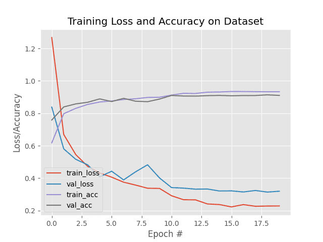
By looking at how close the training and validation metrics evolved throughout, we can safely say that our model didn’t overfit.

Data Distributed Training inference

Although we have already evaluated the model on our test set, we will create a separate script, distributed_inference.py, where we will individually assess test images one by one instead of a full batch at a time.

# USAGE
# python distributed_inference.py

# import the necessary packages
from pyimagesearch.food_classifier import FoodClassifier
from pyimagesearch import config
from pyimagesearch import create_dataloaders
from torchvision import models
from torchvision import transforms
import matplotlib.pyplot as plt
from torch import nn
import torch

# determine the number of GPUs we have
NUM_GPU = torch.cuda.device_count()
print(f"[INFO] number of GPUs found: {NUM_GPU}...")

# determine the batch size based on the number of GPUs
BATCH_SIZE = config.PRED_BATCH_SIZE * NUM_GPU
print(f"[INFO] using a batch size of {BATCH_SIZE}...")

# define augmentation pipeline
testTransform = transforms.Compose([
	transforms.Resize((config.IMAGE_SIZE, config.IMAGE_SIZE)),
	transforms.ToTensor(),
	transforms.Normalize(mean=config.MEAN, std=config.STD)
])

Before initializing the iterators, we set up the initial requirements for these scripts. These include setting up the batch size dictated by the number of CUDA GPUs (Lines 15-19) and initializing a torchvision.transforms instance for our test dataset (Lines 23-27).

# calculate the inverse mean and standard deviation
invMean = [-m/s for (m, s) in zip(config.MEAN, config.STD)]
invStd = [1/s for s in config.STD]

# define our denormalization transform
deNormalize = transforms.Normalize(mean=invMean, std=invStd)

# create test data loader
(testDS, testLoader) = create_dataloaders.get_dataloader(config.TEST,
	transforms=testTransform, bs=BATCH_SIZE, shuffle=True)

# load up the DenseNet121 model
baseModel = models.densenet121(pretrained=True)

# initialize our food classifier
model = FoodClassifier(baseModel, len(testDS.classes))

# load the model state
model.load_state_dict(torch.load(config.MODEL_PATH))

It is important to understand why we are calculating the inverse mean and inverse standard deviation values on Lines 30 and 31. This is because our torchvision.transforms instance normalizes the dataset before it is plugged into the model. So, to turn the image back to its original form, we are calculating these values beforehand. We’ll see how these are used pretty soon!

With these values, we create a torchvision.transforms.Normalize instance for later use (Line 34). Next, we create our test dataset and data loaders using the create_dataloaders method on Lines 37 and 38.

Note that we had saved the trained model state in train_distributed.py. Next, we’ll initialize the model as we had done in the training script (Lines 41-44) and use the model.load_state_dict function to plug in the trained model weights into the initialized model (Line 47).

# if we have more than one GPU then parallelize the model
if NUM_GPU > 1:
	model = nn.DataParallel(model)

# move the model to the device and set it in evaluation mode
model.to(config.DEVICE)
model.eval()

# grab a batch of test data
batch = next(iter(testLoader))
(images, labels) = (batch[0], batch[1])

# initialize a figure
fig = plt.figure("Results", figsize=(10, 10 * NUM_GPU))

We repeat parallelizing the model using nn.DataParallel and set the model to evaluation mode (Lines 50-55). Since we’ll be working with individual data points, we won’t be needing to loop over the full test dataset. Instead, we’ll just grab a batch of test data using next(iter(loader)) (Lines 58 and 59). You can run this function (till the generator runs out of batches) to randomize the batch choice.

# switch off autograd
with torch.no_grad():
	# send the images to the device
	images = images.to(config.DEVICE)

	# make the predictions
	preds = model(images)

	# loop over all the batch
	for i in range(0, BATCH_SIZE):
		# initialize a subplot
		ax = plt.subplot(BATCH_SIZE, 1, i + 1)

		# grab the image, de-normalize it, scale the raw pixel
		# intensities to the range [0, 255], and change the channel
		# ordering from channels first to channels last
		image = images[i]
		image = deNormalize(image).cpu().numpy()
		image = (image * 255).astype("uint8")
		image = image.transpose((1, 2, 0))

		# grab the ground truth label
		idx = labels[i].cpu().numpy()
		gtLabel = testDS.classes[idx]

		# grab the predicted label
		pred = preds[i].argmax().cpu().numpy()
		predLabel = testDS.classes[pred]

		# add the results and image to the plot
		info = "Ground Truth: {}, Predicted: {}".format(gtLabel,
			predLabel)
		plt.imshow(image)
		plt.title(info)
		plt.axis("off")

	# show the plot
	plt.tight_layout()
	plt.show()

Again, since we have no intention of changing the weights of our model, we turn off automatic gradients (Line 65) and flash the test images into our device(s). Finally, on Line 70, we directly make our model predictions on the images in the batch.

Looping over the images in the batch, we select individual images, denormalize them, scale up their values and change their dimension order (Lines 80-83). Changing dimensions is necessary if we display the image because PyTorch chose to design its modules to take channel first inputs. Meaning, our image fresh out of torchvision.transforms is currently Channels * Height * Width. To display it, we have to rearrange the dimensions in the form Height * Width * Channels.

We use the individual label of the image to get the name of the class using testDS.classes (Lines 86 and 87). Next, we get the individual image’s predicted class (Lines 90 and 91). Finally, we compare the real and predicted labels for the individual image (Lines 94-98).

This concludes our inference script for Data Parallel training!

PyTorch Visualizations of Data Parallel Trained Model

Let’s look at a few results plotted by our inference script distributed_inference.py.

As we had taken a batch size of 4 in our inference script, our plot will show pictures of the present batch.

The batch of data sent to our inference script contains: an image of oyster shells (Figure 6), an image of french fries (Figure 7), an image containing meat (Figure 8), and an image of a chocolate cake (Figure 9).

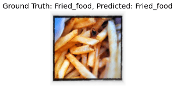
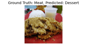
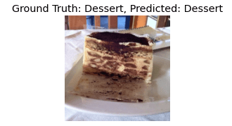
Here we see 3 predictions correct out of a possible 4. This, along with our complete test set scores, tells us that using PyTorch’s data parallel worked pretty nicely!

Summary

In today’s tutorial, we got a little taste of one of PyTorch’s vast array of Distributed Training procedures. The nn.DataParallel may not be the most efficient or fastest among other Distributed Training procedures in terms of internal workings, but it sure is a great place to start! It’s easy to understand and takes only a single line of code to implement. As I mentioned before, the other procedures require more coding, but they were created to handle things more efficiently.

Some very evident problems with nn.DataParallel would be:

• the redundancy of creating entire model instances itself
• failing to work when the model becomes too big to fit
• having no way of adaptively adjusting training when the GPUs available are different

Especially when dealing with a big architecture, model parallelism is preferred, where you can split layers of models among the GPUs.

With that being said, if you are someone who owns multiple GPUs in your system, make use of every bit of computational power your system can provide using nn.DataParallel.

I hope you found this tutorial was helpful enough to pave the way for your curiosity in mastering Distributed Training as a whole!

Citation Information

Chakraborty, D. “Introduction to Distributed Training in PyTorch,” PyImageSearch, 2021, https://pyimagesearch.com/2021/10/18/introduction-to-distributed-training-in-pytorch/

@article{Chakraborty_2021_Distributed, author = {Devjyoti Chakraborty}, title = {Introduction to Distributed Training in {PyTorch}}, journal = {PyImageSearch}, year = {2021}, note = {https://pyimagesearch.com/2021/10/18/introduction-to-distributed-training-in-pytorch/}, }

To download the source code to this post (and be notified when future tutorials are published here on PyImageSearch), simply enter your email address in the form below!