Table of Contents
Introduction to the DeepSeek-V3 Model
The landscape of large language models has been rapidly evolving, with innovations in architecture, training efficiency, and inference optimization pushing the boundaries of what is possible in natural language processing. The DeepSeek-V3 model represents a significant milestone in this evolution, introducing a suite of cutting-edge techniques that address some of the most pressing challenges in modern language model development:
- memory efficiency during inference
- computational cost during training
- effective capture of long-range dependencies
In this comprehensive lesson, we embark on an ambitious journey to build DeepSeek-V3 from scratch, implementing every component from first principles. This isn’t just another theoretical overview. We will write actual, working code that you can run, modify, and experiment with. By the end of this series, you will have a deep understanding of 4 revolutionary architectural innovations and how they synergistically combine to create a powerful language model.
This lesson is the 1st in a 6-part series on Building DeepSeek-V3 from Scratch:
- DeepSeek-V3 Model: Theory, Config, and Rotary Positional Embeddings (this tutorial)
- Lessons 2
- Lesson 3
- Lesson 4
- Lesson 5
- Lesson 6
To learn about DeepSeek-V3 and build it from scratch, just keep reading.
The Four Pillars of DeepSeek-V3
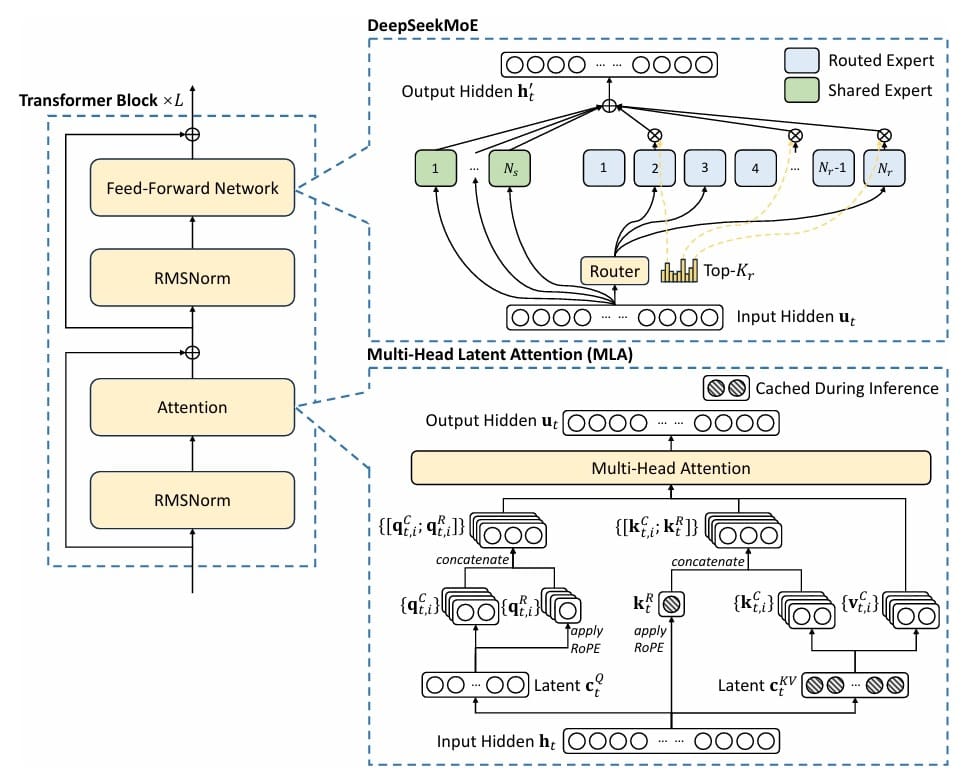
Multihead Latent Attention (MLA): Traditional Transformer models face a critical bottleneck during inference: the key-value (KV) cache grows linearly with sequence length, consuming massive amounts of memory. For a model with 32 attention heads and a hidden dimension of 4096, storing keys and values for a single sequence of 2048 tokens requires over 1GB of memory. DeepSeek’s MLA addresses this by introducing a clever compression-decompression mechanism inspired by Low-Rank Adaptation (LoRA). Instead of storing full key and value matrices, MLA compresses them into a low-rank latent space, achieving up to a 75% reduction in KV cache memory while maintaining model quality. This isn’t just a theoretical improvement; it translates directly to the ability to serve more concurrent users or process longer contexts with the same hardware (Figure 1).
Mixture of Experts (MoE): The challenge in scaling language models is balancing capacity with computational cost. Simply making models wider and deeper becomes prohibitively expensive. MoE offers an elegant solution: instead of every token passing through the same feedforward network, we create multiple “expert” networks and route each token to only a subset of them. DeepSeek-V3 implements this with a learned routing mechanism that dynamically selects the most relevant experts for each token. With 4 experts and top-2 routing, we effectively quadruple the model’s capacity while only doubling the computation per token. The routing function learns to specialize different experts for different types of patterns — perhaps one expert becomes good at handling numerical reasoning, another at processing dialogue, and so on.
Multi-Token Prediction (MTP): Traditional language models predict one token at a time, receiving a training signal only for the immediate next token. This is somewhat myopic — humans don’t just think about the very next word; we plan ahead, considering how sentences and paragraphs will unfold. MTP addresses this by training the model to predict multiple future tokens simultaneously. If we are at position  in the sequence, standard training predicts token
  . MTP adds auxiliary prediction heads that predict tokens
  ,
,  , and so on. This provides a richer training signal, encouraging the model to learn better long-range planning and coherence. It is particularly valuable for tasks requiring forward-looking reasoning.
Rotary Positional Embeddings (RoPE): Transformers don’t inherently understand position — they need explicit positional information. Early approaches used absolute position embeddings, but these struggle with sequences longer than those seen during training. RoPE takes a geometric approach: it rotates query and key vectors in a high-dimensional space, with the rotation angle proportional to the position. This naturally encodes relative position information and exhibits remarkable extrapolation properties. A model trained on 512-token sequences can often handle 2048-token sequences at inference time without degradation.
The combination of these 4 techniques is more than the sum of its parts. MLA reduces memory pressure, allowing us to handle longer contexts or larger batch sizes. MoE increases model capacity without proportional compute increases, making training more efficient. MTP provides richer gradients, accelerating learning and improving model quality. RoPE enables better position understanding and length generalization. Together, they create a model that is efficient to train, efficient to serve, and capable of producing high-quality outputs.
What You Will Build
By the end of this series, you will have implemented a working DeepSeek-V3 model trained on the TinyStories dataset — a curated collection of simple children’s stories. The dataset is ideal for demonstrating core language modeling concepts without requiring massive computational resources. Your model will be able to generate coherent, creative stories in the style of children’s literature. More importantly, you will understand every line of code, every architectural decision, and every mathematical principle behind the model.
The DeepSeek-V3 model we build uses carefully chosen hyperparameters for educational purposes:
- 6 Transformer layers
- 256-dimensional token embeddings
- 8 attention heads
- 4 MoE experts with top-2 routing
- 2-token-ahead prediction training objective (MTP)
These choices balance pedagogical clarity with practical performance: the model is small enough to train on a single GPU in a reasonable time, yet large enough to generate meaningful outputs and demonstrate the key architectural innovations.
Prerequisites and Setup for Building the DeepSeek-V3 Model
Before we dive in, ensure you have a working Python environment with PyTorch 2.0+, the transformers library, and standard scientific computing packages (e.g., numpy, datasets). A GPU is highly recommended but not required — you can train on a CPU, though it will be slower. The complete code is available as a Jupyter notebook, allowing you to experiment interactively.
# Install required packages
!pip install -q transformers datasets torch accelerate tensorboard

# Import core libraries
import os
import math
import torch
import torch.nn as nn
import torch.nn.functional as F
from dataclasses import dataclass
from typing import Optional, Tuple, List, Dict
import logging
import json

print(f"PyTorch version: {torch.__version__}")
print(f"CUDA available: {torch.cuda.is_available()}")
print(f"Device: {torch.device('cuda' if torch.cuda.is_available() else 'cpu')}")
Implementing DeepSeek-V3 Model Configuration and RoPE
DeepSeek-V3 Model Parameters and Configuration
Before we can build any neural network, we need a systematic way to manage its hyperparameters — the architectural decisions that define the model. In modern deep learning, the configuration pattern has become essential: we encapsulate all hyperparameters in a single, serializable object that can be saved, loaded, and modified independently of the model code. This is not just good software engineering — it is crucial for reproducibility, experimentation, and deployment.
DeepSeek-V3’s configuration must capture parameters across multiple dimensions. First, there are the standard Transformer parameters:
- vocabulary size

- number of Transformer layers

- hidden dimension

- number of attention heads

- maximum context length


These follow from the canonical Transformer architecture, where the model transforms input sequences through  layers of self-attention and feedforward processing.
Beyond these basics, we need parameters specific to the DeepSeek-V3 innovations. For MLA, we require the LoRA ranks for key-value compression ( ) and query compression (
 ), as well as the RoPE dimension (
 ). For MoE, we specify the number of experts (
 ), how many to activate per token (
 ), and coefficients for auxiliary losses. For MTP, we define how many tokens ahead to predict (
 ).
).
The mathematical relationship between these parameters determines the model’s computational and memory characteristics. The standard Transformer attention complexity scales as ") for sequence length
for sequence length  . With MLA’s compression, we reduce the KV cache from
  to approximately
  , where
  . For our chosen parameters with
  and
and  , this represents approximately a 50% reduction in KV cache size.
Rotary Positional Embeddings: Geometric Position Encoding
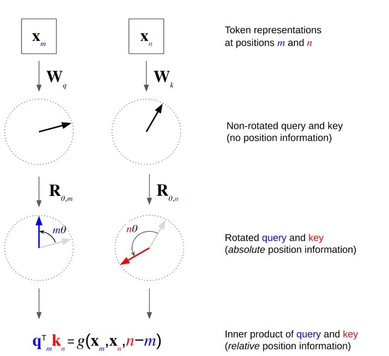
RoPE (Figure 2) represents one of the most elegant ideas in modern Transformer research. To understand it, we must first examine why position matters and where earlier approaches had limitations.
The Position Problem: Self-attention mechanisms are permutation-invariant — if we shuffle the input tokens, we get the same output (modulo the shuffling). But language is sequential; “The cat chased the mouse” means something very different from “The mouse chased the cat.” We need to inject positional information.
Absolute Positional Embeddings: The original Transformer used sinusoidal positional embeddings: } = \sin(\text{pos} / 10000^{2i/d_\text{model}})") and
and } = \cos(\text{pos} / 10000^{2i/d_\text{model}})") . These are added to input embeddings. Learned absolute positional embeddings are another option. But both struggle with extrapolation — a model trained on sequences up to length 512 often fails when applied to sequences of length 1024.
. These are added to input embeddings. Learned absolute positional embeddings are another option. But both struggle with extrapolation — a model trained on sequences up to length 512 often fails when applied to sequences of length 1024.
Relative Position Approaches: Some models (e.g., Transformer-XL) use relative positional encodings, explicitly modeling the distance between tokens. This helps with extrapolation but adds computational overhead.
RoPE’s Geometric Insight: RoPE takes a different approach, encoding position through rotation in complex space. Consider the attention score between query  at position
  and key at position
  :
:

RoPE modifies this by rotating both and by angles proportional to their positions:
^T (R_{\theta, n} k) = q^T R_{\theta, m}^T R_{\theta, n} k = q^T R_{\theta, n-m} k")
where  is the rotation matrix corresponding to position
  . The key insight: rotation matrices satisfy
  , so the attention score naturally depends on the relative position
  rather than absolute positions.
In practice, we implement this in 2D rotation pairs. For a  -dimensional vector, we split it into
  pairs and rotate each pair:
 & -\sin(m\theta_i) \ \sin(m\theta_i) & \cos(m\theta_i) \end{bmatrix} \begin{bmatrix} q_i \ q_{i+1} \end{bmatrix}")
where  follows the same frequency pattern as sinusoidal embeddings. This gives us multiple rotation frequencies, allowing the model to capture both fine-grained and coarse-grained positional relationships.
Why RoPE Extrapolates Well: The rotation formulation naturally extends to positions beyond training data. If the model learns that a relative position of +5 corresponds to a certain rotation angle, it can apply the same principle to positions beyond its training range. The continuous nature of trigonometric functions means there are no discrete position embeddings that “run out.”
RMSNorm: A Modern Normalization Choice: Before diving into code, we should mention RMSNorm (Root Mean Square Normalization), which DeepSeek uses instead of LayerNorm. While LayerNorm computes:
 = \gamma \dfrac{x - \mu}{\sqrt{\sigma^2 + \epsilon}} + \beta")
RMSNorm simplifies by removing the mean-centering and bias:
 = \gamma \dfrac{x}{\sqrt{\dfrac{1}{d}\sum_{i=1}^{d} x_i^2 + \epsilon}}")
This is computationally cheaper and empirically performs just as well for language models. The key insight is that the mean-centering term in LayerNorm may not be necessary for Transformers, where the activations are already roughly centered.
Implementation: Configuration and Rotary Positional Embeddings
Now let’s implement these concepts. We’ll start with the configuration class:
import json


@dataclass
class DeepSeekConfig:
    """Configuration for DeepSeek model optimized for children's stories"""
    vocab_size: int = 50259  # GPT-2 vocabulary size + <|story|> + </|story|> tokens
    n_layer: int = 6         # Number of transformer blocks
    n_head: int = 8          # Number of attention heads
    n_embd: int = 256        # Embedding dimension
    block_size: int = 1024   # Maximum context window
    dropout: float = 0.1     # Dropout rate
    bias: bool = True        # Use bias in linear layers

    # MLA (Multihead Latent Attention) config
    kv_lora_rank: int = 128  # LoRA rank for key-value projection
    q_lora_rank: int = 192   # LoRA rank for query projection
    rope_dim: int = 64       # RoPE dimension

    # MoE (Mixture of Experts) config
    n_experts: int = 4       # Number of experts
    n_experts_per_token: int = 2  # Number of experts per token (top-k)
    expert_intermediate_size: int = 512  # Expert hidden size
    shared_expert_intermediate_size: int = 768  # Shared expert hidden size
    use_shared_expert: bool = True  # Enable shared expert
    aux_loss_weight: float = 0.0  # Auxiliary loss weight (0.0 for aux-free)

    # Multi-token prediction
    multi_token_predict: int = 2  # Predict next 2 tokens
Lines 1-5: Configuration Class Structure: We use Python’s @dataclass decorator to define our DeepSeekConfig class, which automatically generates initialization and representation methods. This is more than syntactic sugar — it ensures type hints are respected and provides built-in equality comparisons. The configuration serves as a single source of truth for model hyperparameters, making it easy to experiment with different architectures by simply modifying this object.
Lines 7-13: Standard Transformer Parameters: We define the core Transformer dimensions. The vocabulary size of 50,259 comes from the GPT-2 tokenizer, with two additional custom tokens for story boundaries. We choose 6 layers and a 256-dimensional embedding size as a balance between model capacity and computational cost — this is small enough to train on a single consumer GPU but large enough to demonstrate the key DeepSeek innovations. The block size of 1024 determines the model’s maximum context length, sufficient for coherent short stories. The dropout rate of 0.1 provides regularization without being overly aggressive.
Lines 16-18: MLA Configuration: These parameters control our Multihead Latent Attention mechanism. The kv_lora_rank of 128 means we compress key-value representations from 256 dimensions down to 128 — a 50% reduction that translates directly to KV cache memory savings. The q_lora_rank of 192 provides slightly more capacity for query compression since queries don’t need to be cached during inference. The rope_dim of 64 specifies how many dimensions use RoPE — we don’t apply RoPE to all dimensions, only to a subset, allowing some dimensions to focus purely on content rather than position.
Lines 21-29: MoE and MTP Configuration: We configure 4 expert networks with top-2 routing, meaning each token will be processed by exactly 2 out of 4 experts. This gives us 2× more parameters than a standard feedforward layer while maintaining the same computational cost. The aux_loss_weight of 0.01 determines how strongly we penalize uneven expert usage — this is crucial for preventing all tokens from routing to just one or two experts. The multi_token_predict parameter determines how many future tokens the model is trained to predict at each step.
    def __post_init__(self):
        """Initialize special tokens after dataclass initialization"""
        self.special_tokens = {
            "story_start": "<|story|>",
            "story_end": "</|story|>",
        }

    def to_dict(self):
        """Convert configuration to dictionary"""
        return {
            'vocab_size': self.vocab_size,
            'n_layer': self.n_layer,
            'n_head': self.n_head,
            'n_embd': self.n_embd,
            'block_size': self.block_size,
            'dropout': self.dropout,
            'bias': self.bias,
            'kv_lora_rank': self.kv_lora_rank,
            'q_lora_rank': self.q_lora_rank,
            'rope_dim': self.rope_dim,
            'n_experts': self.n_experts,
            'n_experts_per_token': self.n_experts_per_token,
            'expert_intermediate_size': self.expert_intermediate_size,
            'shared_expert_intermediate_size': self.shared_expert_intermediate_size,
            'use_shared_expert': self.use_shared_expert,
            'aux_loss_weight': self.aux_loss_weight,
            'multi_token_predict': self.multi_token_predict,
            'special_tokens': self.special_tokens,
        }

    def to_json_string(self, indent=2):
        """Convert configuration to JSON string"""
        return json.dumps(self.to_dict(), indent=indent)

    @classmethod
    def from_dict(cls, config_dict):
        """Create configuration from dictionary"""
        # Remove special_tokens from dict as it's set in __post_init__
        config_dict = {k: v for k, v in config_dict.items() if k != 'special_tokens'}
        return cls(**config_dict)

    @classmethod
    def from_json_string(cls, json_string):
        """Create configuration from JSON string"""
        return cls.from_dict(json.loads(json_string))
Lines 31-75: Special Methods for Serialization: We implement __post_init__ to add special tokens after initialization, ensuring they’re always present but not required in the constructor. The to_dict and to_json_string methods enable easy serialization for saving configurations alongside trained models. The class methods from_dict and from_json_string provide deserialization, creating a complete round-trip for configuration management. This pattern is essential for reproducibility — we can save a configuration with our trained model and later reconstruct the exact architecture.
Next, we implement the RoPE module.
class RMSNorm(nn.Module):
    """Root Mean Square Layer Normalization"""
    def __init__(self, ndim, eps=1e-6):
        super().__init__()
        self.eps = eps
        self.weight = nn.Parameter(torch.ones(ndim))

    def forward(self, x):
        norm = x.norm(dim=-1, keepdim=True) * (x.size(-1) ** -0.5)
        return self.weight * x / (norm + self.eps)
RMSNorm Implementation (Lines 1-10): Our RMSNorm class is remarkably simple. In the constructor, we create a learnable weight parameter (the  in our equations) initialized to ones. In the forward pass, we compute the L2 norm of the input along the feature dimension, multiply by
  to get the RMS, and then scale the input by the inverse of this norm (plus epsilon for numerical stability) and multiply by the learned weight parameter. This normalization ensures our activations have unit RMS, helping with training stability and gradient flow.
class RotaryEmbedding(nn.Module):
    """Rotary Positional Embedding (RoPE) for better position understanding"""
    def __init__(self, dim, max_seq_len=2048):
        super().__init__()
        inv_freq = 1.0 / (10000 ** (torch.arange(0, dim, 2).float() / dim))
        self.register_buffer('inv_freq', inv_freq)
        self.max_seq_len = max_seq_len

    def forward(self, x, seq_len=None):
        if seq_len is None:
            seq_len = x.shape[-2]

        t = torch.arange(seq_len, device=x.device).type_as(self.inv_freq)
        freqs = torch.outer(t, self.inv_freq)
        cos, sin = freqs.cos(), freqs.sin()
        return cos, sin

def apply_rope(x, cos, sin):
    """Apply rotary position embedding"""
    x1, x2 = x.chunk(2, dim=-1)
    return torch.cat([x1 * cos - x2 * sin, x1 * sin + x2 * cos], dim=-1)
The RotaryEmbedding Class (Lines 12-27): The constructor creates the inverse frequency vector inv_freq following the same frequency schedule used in sinusoidal positional embeddings, where each pair of dimensions is assigned a frequency following the schedule  . We use
 register_buffer rather than a parameter because these frequencies shouldn’t be learned — they’re fixed by our positional encoding design. In the forward pass, we create position indices from 0 to seq_len, compute the outer product with inverse frequencies (giving us a matrix where entry ") is
is  , and compute the cosine and sine values. These will be broadcast and applied to query and key vectors. The resulting cosine and sine tensors broadcast across the batch, head, and sequence dimensions during attention computation.
The apply_rope Function (Lines 29-32): This elegant function applies the 2D rotation. We chunk the input into pairs of dimensions (effectively treating each pair of dimensions as the real and imaginary components of a complex number). We then apply the rotation formula:
 = (x_1 \cos \theta - x_2 \sin \theta, x_1 \sin \theta + x_2 \cos \theta).")
The chunking operation splits along the last dimension. We compute each rotated component and then concatenate them back together. This vectorized implementation is far more efficient than iterating over dimension pairs in Python.
Design Choices and Tradeoffs: Several decisions merit discussion. We chose partial RoPE (rope_dim=64 rather than full n_embd=256) because empirical research shows that applying RoPE to all dimensions can sometimes hurt performance — some dimensions benefit from remaining content-focused rather than encoding position. Our LoRA ranks are fairly high (128 and 192) relative to the 256-dimensional embeddings; in larger models, the compression ratio would be more aggressive. The special tokens pattern (story_start and story_end) provides explicit boundaries that help the model learn story structure — it knows when a generation should terminate.
What's next? We recommend PyImageSearch University.

86+ total classes • 115+ hours hours of on-demand code walkthrough videos • Last updated: March 2026
★★★★★ 4.84 (128 Ratings) • 16,000+ Students Enrolled
I strongly believe that if you had the right teacher you could master computer vision and deep learning.
Do you think learning computer vision and deep learning has to be time-consuming, overwhelming, and complicated? Or has to involve complex mathematics and equations? Or requires a degree in computer science?
That’s not the case.
All you need to master computer vision and deep learning is for someone to explain things to you in simple, intuitive terms. And that’s exactly what I do. My mission is to change education and how complex Artificial Intelligence topics are taught.
If you're serious about learning computer vision, your next stop should be PyImageSearch University, the most comprehensive computer vision, deep learning, and OpenCV course online today. Here you’ll learn how to successfully and confidently apply computer vision to your work, research, and projects. Join me in computer vision mastery.
Inside PyImageSearch University you'll find:
- ✓ 86+ courses on essential computer vision, deep learning, and OpenCV topics
- ✓ 86 Certificates of Completion
- ✓ 115+ hours hours of on-demand video
- ✓ Brand new courses released regularly, ensuring you can keep up with state-of-the-art techniques
- ✓ Pre-configured Jupyter Notebooks in Google Colab
- ✓ Run all code examples in your web browser — works on Windows, macOS, and Linux (no dev environment configuration required!)
- ✓ Access to centralized code repos for all 540+ tutorials on PyImageSearch
- ✓ Easy one-click downloads for code, datasets, pre-trained models, etc.
- ✓ Access on mobile, laptop, desktop, etc.
Summary
In this blog, we walk through the foundations of DeepSeek-V3, starting with its theoretical underpinnings and the four pillars that shape its architecture. We explore why these pillars matter, how they guide the design of the model, and what we aim to build by the end of the lesson. By laying out the prerequisites and setup, we ensure that we’re equipped with the right tools and mindset before diving into the implementation details.
Next, we focus on the model configuration, where we break down the essential parameters that define DeepSeek-V3’s behavior. We discuss how these configurations influence performance, scalability, and adaptability, and why they are critical for building a robust model. Alongside this, we introduce Rotary Positional Embeddings (RoPE), a geometric approach to positional encoding that enhances the model’s ability to capture sequential information with precision.
Finally, we bring theory into practice by implementing both the configuration and RoPE step by step. We highlight how these components integrate seamlessly, forming the backbone of DeepSeek-V3. By the end, we not only understand the theoretical aspects but also gain hands-on experience in building and customizing the model. Together, these steps demystify the process and set the stage for deeper experimentation with advanced Transformer architectures.
Citation Information
Mangla, P. “DeepSeek-V3 Model: Theory, Config, and Rotary Positional Embeddings,” PyImageSearch, S. Huot, A. Sharma, and P. Thakur, eds., 2026, https://pyimg.co/1atre
@incollection{Mangla_2026_deepseek-v3-model-theory-config-and-rotary-positional-embeddings,
  author = {Puneet Mangla},
  title = {{DeepSeek-V3 Model: Theory, Config, and Rotary Positional Embeddings}},
  booktitle = {PyImageSearch},
  editor = {Susan Huot and Aditya Sharma and Piyush Thakur},
  year = {2026},
  url = {https://pyimg.co/1atre},
}
To download the source code to this post (and be notified when future tutorials are published here on PyImageSearch), simply enter your email address in the form below!

Download the Source Code and FREE 17-page Resource Guide
Enter your email address below to get a .zip of the code and a FREE 17-page Resource Guide on Computer Vision, OpenCV, and Deep Learning. Inside you'll find my hand-picked tutorials, books, courses, and libraries to help you master CV and DL!

Comment section
Hey, Adrian Rosebrock here, author and creator of PyImageSearch. While I love hearing from readers, a couple years ago I made the tough decision to no longer offer 1:1 help over blog post comments.
At the time I was receiving 200+ emails per day and another 100+ blog post comments. I simply did not have the time to moderate and respond to them all, and the sheer volume of requests was taking a toll on me.
Instead, my goal is to do the most good for the computer vision, deep learning, and OpenCV community at large by focusing my time on authoring high-quality blog posts, tutorials, and books/courses.
If you need help learning computer vision and deep learning, I suggest you refer to my full catalog of books and courses — they have helped tens of thousands of developers, students, and researchers just like yourself learn Computer Vision, Deep Learning, and OpenCV.
Click here to browse my full catalog.