Object Detection in Gaming: Fine-Tuning Google’s PaliGemma 2 for Valorant

---

---

Object Detection in Gaming: Fine-Tuning Google’s PaliGemma 2 for Valorant

In our previous 4-part series, we explored PaliGemma in depth — covering its architecture, fine-tuning, and various tasks it can perform. We built interactive applications using Gradio and deployed them on Hugging Face Spaces, making them easily accessible. We also demonstrated a simple object detection demo using an interactive Gradio application.

Since object detection plays a crucial role in real-world applications, we are launching a 2-part series on Object Detection with Google’s PaliGemma 2 Model, where we will fine-tune the pre-trained PaliGemma 2 model for specialized tasks across different industries.

In this first tutorial, we will fine-tune the PaliGemma 2 model to detect objects in Valorant, a popular FPS (first-person shooter) game, showcasing how object detection can enhance gameplay insights.

Note: The implementation steps remain the same for both the PaliGemma 1 and PaliGemma 2 models.

This lesson is the 1st in a 2-part series on Vision-Language Models — Object Detection:

1. Object Detection in Gaming: Fine-Tuning Google’s PaliGemma 2 for Valorant (this tutorial)
2. AI for Healthcare: Fine-Tuning Google’s PaliGemma 2 for Brain Tumor Detection

Moreover, we will also provide a bonus code to our PyImageSearch University Members for detecting hazards in construction sites following the same implementation steps at the end of the 2nd blog post.

To learn how to fine-tune the PaliGemma 2 model for detecting Valorant Objects, just keep reading.

---

How would you like immediate access to 3,457 images curated and labeled with hand gestures to train, explore, and experiment with … for free? Head over to Roboflow and get a free account to grab these hand gesture images.

---

Configuring Your Development Environment

To follow this guide, you need to have the following libraries installed on your system.

!pip install -q datasets transformers peft bitsandbytes

We install datasets to load and process datasets, transformers to load the PaliGemma model, peft to enable parameter-efficient fine-tuning for optimizing large models, and bitsandbytes for memory-efficient model loading through quantization.

In order to load the model from Hugging Face, we need to:

• Set up your Hugging Face Access Token
• Set up your Colab Secrets to Access Hugging Face Resources
• Grant Permission to Access the PaliGemma Model

Please refer to the following blog post to complete the setup: Configure Your Hugging Face Access Token in Colab Environment.

---

Need Help Configuring Your Development Environment?

All that said, are you:

• Short on time?
• Learning on your employer’s administratively locked system?
• Wanting to skip the hassle of fighting with the command line, package managers, and virtual environments?
• Ready to run the code immediately on your Windows, macOS, or Linux system?

Then join PyImageSearch University today!

Gain access to Jupyter Notebooks for this tutorial and other PyImageSearch guides pre-configured to run on Google Colab’s ecosystem right in your web browser! No installation required.

And best of all, these Jupyter Notebooks will run on Windows, macOS, and Linux!

---

Setup and Imports

Once we have installed the necessary libraries, we can proceed with importing them.

import torch
import re
import cv2

from PIL import ImageDraw
from IPython.display import display

from datasets import load_dataset
from peft import get_peft_model, LoraConfig

from transformers import Trainer
from transformers import TrainingArguments
from transformers import BitsAndBytesConfig
from transformers import PaliGemmaProcessor, PaliGemmaForConditionalGeneration

We first import torch to handle tensor computations. Next, we bring in the re module for working with regular expressions and cv2 for image processing.

Then, we import ImageDraw from the PIL library to draw bounding boxes on images and display from IPython.display to visualize outputs in the Colab environment.

We use load_dataset from the datasets library to easily load datasets. From peft, we import get_peft_model to apply parameter-efficient fine-tuning (PEFT) and LoraConfig to configure the Low-Rank Adaptation (LoRA) method for optimizing large models.

To simplify model training and evaluation, we import the Trainer class and set up training configurations using TrainingArguments from transformers. Additionally, BitsAndBytesConfig enables quantization for memory-efficient model processing.

Finally, we import PaliGemmaProcessor, which processes image-text inputs, and PaliGemmaForConditionalGeneration, which loads the PaliGemma model for object detection.

---

Load the Valorant Dataset

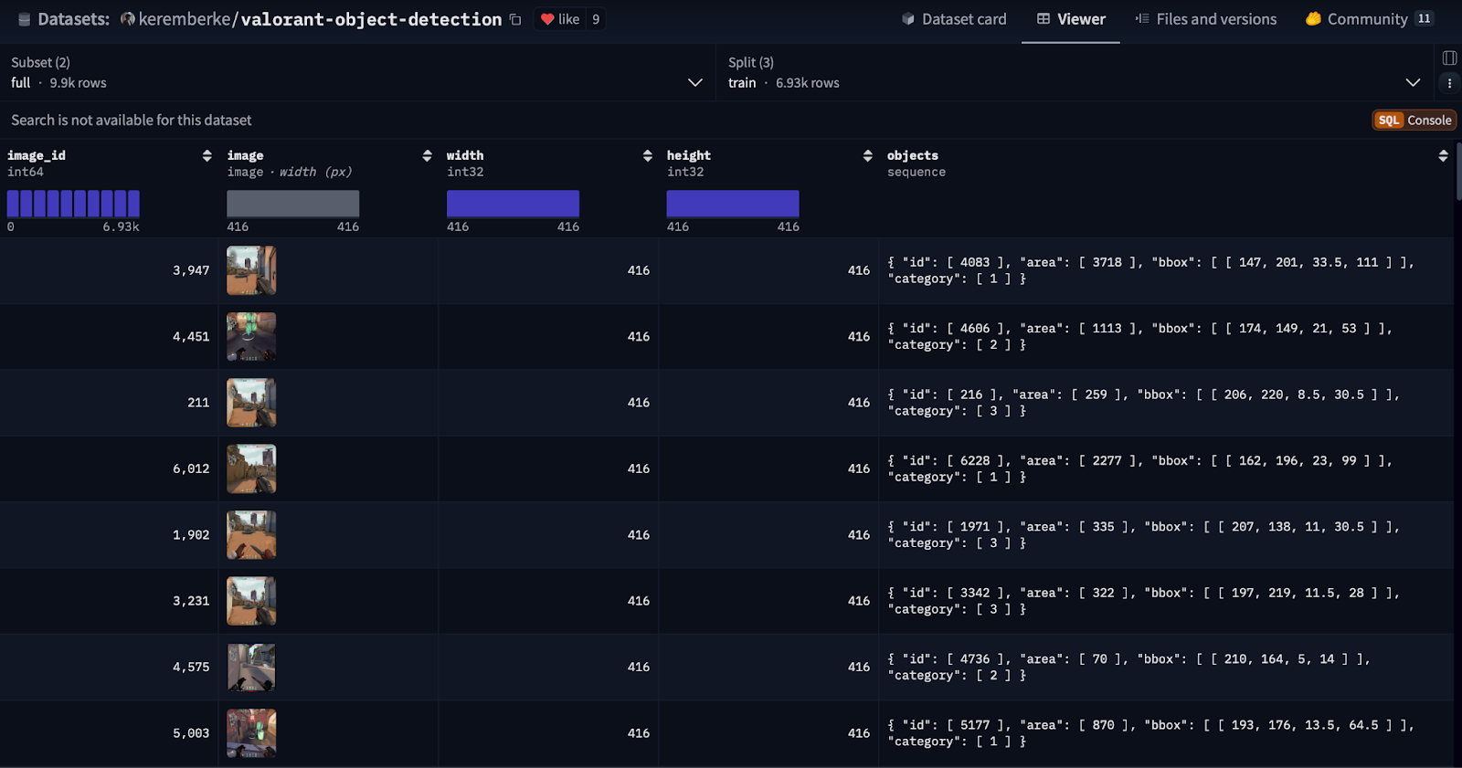
To fine-tune PaliGemma, we need a custom dataset with labeled objects from Valorant. For this, we use the Valorant Object Detection dataset, hosted on Hugging Face, which provides annotated in-game objects for training. The dataset (Figure 1) is available at keremberke/valorant-object-detection.

ds = load_dataset("keremberke/valorant-object-detection", name="full")

We load the dataset using the load_dataset function from the datasets library:

Here’s what happens in this step:

• We call load_dataset, which automatically downloads and prepares the dataset for use.
• We specify "keremberke/valorant-object-detection", which is a pre-existing dataset for detecting in-game objects in Valorant.
• The name="full" argument ensures we load the complete dataset.

ds

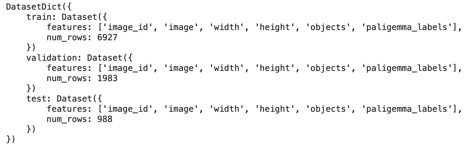
Once we load the dataset, we can examine its structure (Figure 2) to understand how the data is organized. The dataset is loaded as a DatasetDict, which contains three subsets:

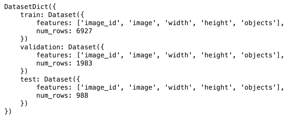
This dataset consists of training, validation, and test splits:

• Train: 6,927 images for training the model.
• Validation: 1,983 images to tune hyperparameters.
• Test: 988 images for evaluating the model’s final performance.

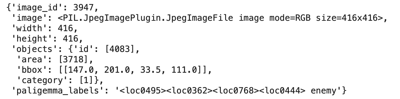
ds["train"][0]

Each data point in the dataset includes an image and its associated metadata. Here’s an example (Figure 3):

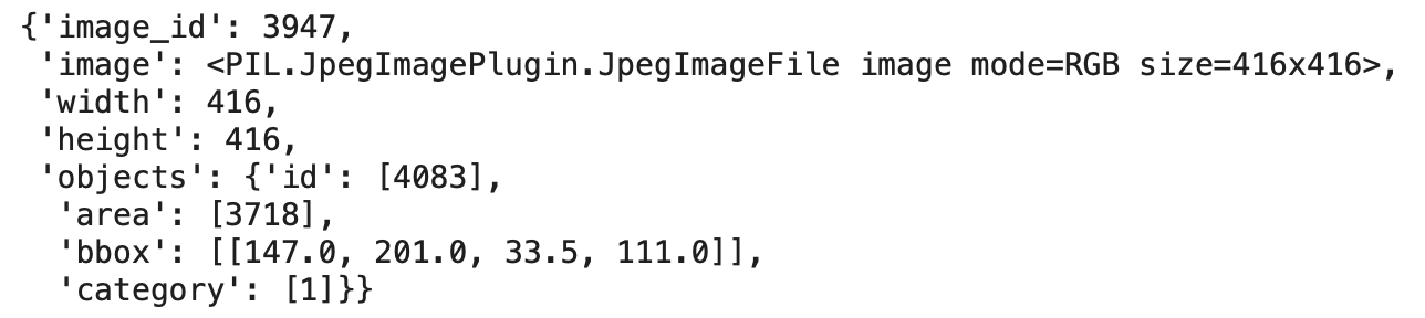
Breaking it down:

• image_id: A unique identifier for the image.
• image: A PIL (Python Imaging Library) image in RGB format with a resolution of 416×416 pixels.
• width and height: The dimensions of the image.
• objects: Contains annotations for objects detected in the image.
  • id: Unique ID for the object.
  • area: The pixel area covered by the object.
  • bbox: Bounding box coordinates [x, y, width, height] specifying the object’s location.
  • category: The class label for the detected object.

---

Format Dataset to PaliGemma Format

When fine-tuning PaliGemma for object detection, the image, bounding box, and its corresponding labels must follow the required format. The image is already provided in PIL format, but the bounding box coordinates and labels need to be converted into PaliGemma’s specific format:

<locXXXX><locXXXX><locXXXX><locXXXX> [CLASS]

The dataset contains object bounding boxes (bbox) and corresponding category indices. The bounding box coordinates are provided in COCO (Common Objects in Context) format:

[x, y, width, height]

where (x, y) represents the top-left corner, and width and height define the size of the bounding box. Additionally, the dataset assigns numerical category indices (0 to 3), each corresponding to a class label:

• 0 → Dropped Spike
• 1 → Enemy
• 2 → Planted Spike
• 3 → Teammate

['dropped spike', 'enemy', 'planted spike', 'teammate']

To prepare the data for PaliGemma, we need to:

Convert COCO-style bounding box coordinates to xyxy format:

[x_min, y_min, x_max, y_max]

where:

• x_min = x
• y_min = y
• x_max = x + width
• y_max = y + height

Normalize these coordinates to a fixed scale and convert them into PaliGemma’s <locXXXX> format.

Construct the final label string in the format:

<locY1><locX1><locY2><locX2> [CLASS]

where the location tags are derived from the normalized bounding box coordinates.

By applying this transformation to the dataset, we ensure that the input labels are compatible with PaliGemma’s expected format for training.

---

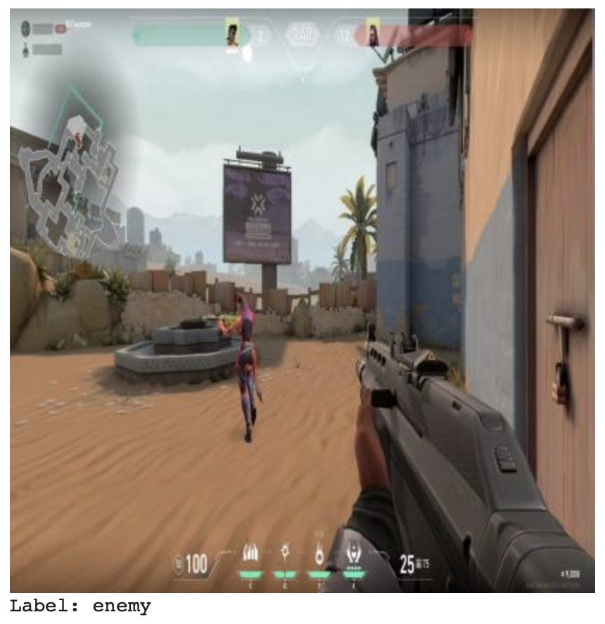
Display Train Image and Label

Let’s first visualize a sample image and label from the training dataset.

# Get the first example from the dataset
example = ds["train"][0]

# Extract the image and objects
image = example["image"]
categories_idx = example["objects"]["category"]  # List of category indices
category_labels = ['dropped spike', 'enemy', 'planted spike', 'teammate']  # Example category names

# Display the image
display(image)

# Display the category names for each object in the image
for idx in categories_idx:
   category_name = category_labels[idx]  # Map the index to the label name
   print(f"Label: {category_name}")

First, retrieve the first example from the dataset.

• The dataset is stored in a dictionary-like format.
• ds["train"][0] accesses the first data sample in the training dataset.

Next, extract the image and object category indices.

• The "image" key stores the image, which is extracted and assigned to the image variable.
• The "objects" key contains metadata about objects present in the image.
• ["objects"]["category"] retrieves a list of indices representing object classes.
• Each index corresponds to a category (e.g., an enemy or a planted spike).

Define the category names for easy interpretation.

• The dataset uses numerical indices to represent object categories.
• This list maps those indices to their corresponding names:
  • 0 → "dropped spike"
  • 1 → "enemy"
  • 2 → "planted spike"
  • 3 → "teammate"
• This mapping allows us to convert category indices into meaningful labels.

Then, we use display(image) from IPython.display to display the image.

Finally, we print the object labels.

• This loop goes through each category index in categories_idx.
• It finds the corresponding label from category_labels using category_labels[idx].
• The label is printed, showing which objects are present in the image.

In Figure 4, we can see the displayed image and the label.

---

COCO Format BBox to XYXY Format

Now, we define a function to convert the bounding box coordinates from COCO format ([x, y, width, height]) to XYXY format ([x1, y1, x2, y2]).

# Function to convert COCO-style bbox to xyxy format
def coco_to_xyxy(coco_bbox):
   x, y, width, height = coco_bbox
   x1, y1 = x, y
   x2, y2 = x + width, y + height
   return [x1, y1, x2, y2]

First, we extract the bounding box coordinates and dimensions. Then, we keep x1, y1 the same (top-left corner) and add width and height to x1, y1 to get the bottom-right corner. Finally, we return the bounding box in XYXY format.

---

Scale Bounding Box Values

In this step, we define a function to scale the bounding box values to a fixed range.

# Function to format location values to a fixed scale
def format_location(value, max_value):
   # Convert normalized location values to integers in the range [0, 1024]
   return f"<loc{int(round(value * 1024 / max_value)):04}>"

First, we take the location value (either x or y coordinate) and the maximum value for that dimension (width or height of the image). Then, we scale the value by multiplying it by 1024 and dividing it by the maximum value, which normalizes the value to a range of [0, 1024]. After that, we round the scaled value and format it as a string, ensuring it’s padded to 4 digits using int(round(...)):04. Finally, we return the formatted string in the format <locXXXX>, where XXXX is the scaled location value.

---

Define Conversion Function

Now, we define a function to convert bounding box coordinates and category labels into PaliGemma format. The goal is to generate labels in the format <locXXXX><locXXXX><locXXXX><locXXXX> [CLASS].

# Function to convert bounding boxes and categories into paligemma format
def convert_to_paligemma_format(bboxs, categories, category_names, image_width, image_height):
   detection_strings = []
   for bbox, category in zip(bboxs, categories):
       x1, y1, x2, y2 = coco_to_xyxy(bbox)  # Convert bbox to xyxy format
       name = category_names[category]  # Use category index to get the name
       locs = [
           format_location(y1, image_height),
           format_location(x1, image_width),
           format_location(y2, image_height),
           format_location(x2, image_width),
       ]
       detection_string = "".join(locs) + f" {name}"
       detection_strings.append(detection_string)

   return " ; ".join(detection_strings)

First, we initialize an empty list, detection_strings, to store formatted object annotations. Then, we loop through each bounding box and its corresponding category label using zip(bboxs, categories). For each bounding box, we convert it from COCO format to XYXY format using the coco_to_xyxy function.

Next, we retrieve the category name from the category_names list using the category index. After that, we scale and format the bounding box coordinates using the format_location function, ensuring that the values are mapped to a fixed range of [0, 1024] and formatted as <locXXXX>. These formatted location values are stored in a list called locs.

Then, we concatenate the location values and append the category name at the end, forming the final detection string for that object. This string is added to the detection_strings list.

Finally, we join all detection strings using ; as a separator and return the formatted annotation string, ensuring multiple objects in an image are properly structured as required by PaliGemma.

---

Define Function to Process Single Dataset Example

Now, we define a function to process a single dataset example and convert its object annotations into PaliGemma format. This function extracts relevant information from the dataset and prepares the label in the required format.

# Function to process a single dataset example
def format_objects(example, category_names):
   height = example["height"]
   width = example["width"]
   bboxs = example["objects"]["bbox"]
   categories = example["objects"]["category"]
   formatted_objects = convert_to_paligemma_format(bboxs, categories, category_names, width, height)
   return {"paligemma_labels": formatted_objects}

First, we retrieve the height and width of the image from the dataset example. Then, we extract the bounding box coordinates (bboxs) and the corresponding category labels (categories) from the "objects" field.

Next, we pass these extracted values to the convert_to_paligemma_format function, along with the category_names list and the image dimensions. This function processes the bounding boxes and categories, returning a formatted string where each object is represented in the <locXXXX><locXXXX><locXXXX><locXXXX> [CLASS] format.

Finally, we return a dictionary containing the key "paligemma_labels" with the formatted string as its value. This ensures that each dataset example now has labels compatible with PaliGemma for training and inference.

---

Apply Formatting

Now, we apply the formatting function to each split of the dataset to ensure that all annotations follow the PaliGemma format.

# Define the category names
category_names = ["dropped spike", "enemy", "planted spike", "teammate"]

# Apply formatting to each split of the dataset
print("[INFO] Processing dataset...")
ds["train"] = ds["train"].map(lambda example: format_objects(example, category_names))
ds["validation"] = ds["validation"].map(lambda example: format_objects(example, category_names))
ds["test"] = ds["test"].map(lambda example: format_objects(example, category_names))

First, we define a list called category_names, which contains the class labels: "dropped spike", "enemy", "planted spike", and "teammate". These labels correspond to the category indices present in the dataset.

Next, we print a message to indicate that the dataset processing has started. Then, we use the .map() function to apply the format_objects function to every example in the training, validation, and test datasets. This ensures that each image’s bounding boxes and category labels are converted into the <locXXXX><locXXXX><locXXXX><locXXXX> [CLASS] format required for PaliGemma.

Finally, after processing, each dataset split (train, validation, and test) will contain the additional "paligemma_labels" field, which holds the formatted annotations ready for model training.

ds

To verify, we can see the dataset structure (Figure 5) again.

We can clearly see that paligemma_labels has been added to all the dataset splits.

ds["train"][0]

Let’s also examine the first sample from the training dataset (Figure 6).

We can clearly see that the paligemma_labels field contains the final formatted label: <loc0495><loc0362><loc0768><loc0444> enemy. Here, the bbox has been converted to the <locXXXX> format followed by its [CLASS], ensuring compatibility with PaliGemma’s requirements. Finally, this confirms that the dataset example is correctly processed and ready for fine-tuning.

---

Push the PaliGemma-Formatted Dataset to the Hugging Face Hub

Now, we push the processed dataset to the Hugging Face Hub for easy access and sharing.

# Push the processed dataset back to the Hugging Face Hub
print("[INFO] Pushing processed dataset to the Hugging Face Hub...")
ds.push_to_hub(
   repo_id= "pyimagesearch/valorant-object-detection-paligemma",
   commit_message= "added valorant object detection paligemma dataset"
)

First, we print a log message to indicate that the dataset upload is starting. Next, we use the push_to_hub method on ds, which contains the formatted dataset. This function uploads the dataset to the specified repository "pyimagesearch/valorant-object-detection-paligemma" on Hugging Face with a commit message "added valorant object detection paligemma dataset".

The PaliGemma-formatted dataset can be found here: pyimagesearch/valorant-object-detection-paligemma

This step ensures that the dataset is publicly available for retrieval and further experimentation.

---

Perform Inference with the Pre-Trained PaliGemma 2 Model

Before fine-tuning, let’s evaluate how the pre-trained PaliGemma 2 model performs in detecting objects in the Valorant game. This helps establish a baseline for comparison after fine-tuning.

---

Load the PaliGemma-Formatted Dataset

Let’s load the PaliGemma-formatted dataset which we have pushed just now.

valorant_od_paligemma_ds = load_dataset("pyimagesearch/valorant-object-detection-paligemma")

We use the same load_dataset function to load the dataset as we did earlier.

valorant_od_paligemma_ds

We verify that the dataset is correctly loaded by printing valorant_od_paligemma_ds.

From Figure 7, we can see a DatasetDict structure, confirming that the dataset contains the expected splits and features.

---

Load the Pre-Trained PaliGemma 2 Model and Processor

Once our dataset is loaded, we load the pre-trained PaliGemma 2 model and processor.

pretrained_model_id = "google/paligemma2-3b-pt-224"

We first define the model (google/paligemma2-3b-pt-224) with 3b parameters and 224×224 image resolution.

pretrained_processor = PaliGemmaProcessor.from_pretrained(pretrained_model_id)

Next, we load the PaliGemmaProcessor using the from_pretrained method to process inputs for the model.

pretrained_model = PaliGemmaForConditionalGeneration.from_pretrained(pretrained_model_id)

Finally, we load the model using the from_pretrained method of PaliGemmaForConditionalGeneration.

---

Parse Multiple Locations

To extract bounding box coordinates and labels from the model’s output, we define a helper function using Regular Expressions (RegEx).

# Helper function to parse multiple <loc> tags and return a list of coordinate sets and labels
def parse_multiple_locations(decoded_output):
   # Regex pattern to match four <locxxxx> tags and the label at the end (e.g., 'cat')
   loc_pattern = r"<loc(\d{4})><loc(\d{4})><loc(\d{4})><loc(\d{4})>\s+([^;]+)"

   matches = re.findall(loc_pattern, decoded_output)
   coords_and_labels = []

   for match in matches:
       # Extract the coordinates and label
       y1 = int(match[0]) / 1024
       x1 = int(match[1]) / 1024
       y2 = int(match[2]) / 1024
       x2 = int(match[3]) / 1024
       label = match[4].strip()

       coords_and_labels.append({
           'label': label,
           'bbox': [y1, x1, y2, x2]
       })

   return coords_and_labels

First, we define a RegEx pattern to detect four <locxxxx> tags, each containing 4-digit coordinates, followed by a label (e.g., 'cat').

Next, we use re.findall() to find all matches in the decoded output. We then initialize an empty list (coords_and_labels) to store the extracted bounding boxes and labels.

After that, we iterate through the matches, extracting four coordinates and converting them from integer format (scaled by 1024) to floating-point values (normalized between 0 and 1).

Finally, we store each label along with its corresponding bounding box coordinates.

The function returns a list of parsed bounding boxes and labels, ready for further processing.

---

Draw Multiple Bounding Boxes

To visualize detected objects, we define a helper function that draws bounding boxes and labels on the input image.

# Helper function to draw bounding boxes and labels for all objects on the image
def draw_multiple_bounding_boxes(image, coords_and_labels):
   draw = ImageDraw.Draw(image)
   width, height = image.size

   for obj in coords_and_labels:
       # Extract the bounding box coordinates
       y1, x1, y2, x2 = obj['bbox'][0] * height, obj['bbox'][1] * width, obj['bbox'][2] * height, obj['bbox'][3] * width

       # Draw bounding box and label
       draw.rectangle([x1, y1, x2, y2], outline="red", width=3)
       draw.text((x1, y1), obj['label'], fill="red")

   return image

First, we initialize ImageDraw.Draw() to allow drawing on the image. We also extract the image dimensions (width, height) for scaling the bounding box coordinates.

Next, we loop through each object, convert normalized coordinates (0-1 range) into pixel values using the image dimensions (multiply the y values by the image height and the x values by the image width to get pixel coordinates), and extract the bounding box coordinates.

After that, we use draw.rectangle() to outline the detected object in red and draw.text() to label it at the top-left corner.

Finally, we return the annotated image with bounding boxes and labels, making object detection results visually interpretable.

---

Define Inference Function

We define an inference function to process an image and a text prompt, extract bounding box information, and return an annotated image with object labels.

# Define inference function
def process_image(image, prompt):
   # Process the image and prompt using the processor
   inputs = pretrained_processor(image.convert("RGB"), prompt, return_tensors="pt")

   try:
       # Generate output from the model
       output = pretrained_model.generate(**inputs, max_new_tokens=100)

       # Decode the output from the model
       decoded_output = pretrained_processor.decode(output[0], skip_special_tokens=True)

       # Extract bounding box coordinates and labels
       coords_and_labels = parse_multiple_locations(decoded_output)

       if coords_and_labels:
           # Draw bounding boxes and labels on the image
           image_with_boxes = draw_multiple_bounding_boxes(image, coords_and_labels)

           # Prepare the coordinates and labels for the UI
           labels_and_coords = "\n".join([f"Label: {obj['label']}, Coordinates: {obj['bbox']}" for obj in coords_and_labels])

           # Return the modified image and the list of coordinates+labels
           return display(image_with_boxes), labels_and_coords
       else:
           return "No bounding boxes detected."

   except IndexError as e:
       print(f"IndexError: {e}")
       return "An error occurred during processing."

First, we convert the image to RGB and process it with the prompt using pretrained_processor, ensuring compatibility with the model.

Next, we generate predictions using pretrained_model.generate, limiting the response to 100 tokens.

We decode the output into a human-readable format using pretrained_processor.decode, excluding special tokens.

Then, we extract bounding box coordinates and labels using the parse_multiple_locations() function defined above.

If objects are detected, we use draw_multiple_bounding_boxes() to overlay bounding boxes and labels on the image.

We format the extracted labels and bounding box coordinates for easy readability.

Finally, we return the annotated image, and extracted bounding boxes and labels for further analysis.

If no bounding boxes are detected, we return a message saying No bounding boxes detected.

If an error occurs, we handle it gracefully, ensuring the function returns a consistent output format.

---

Example 1

Let’s see 1st inference output with the pre-trained PaliGemma 2 model.

---

Display Test Image and Label

# Get the first example from the test dataset
test_example = valorant_od_paligemma_ds["test"][0]

# Extract the image and objects
test_image = test_example["image"]
categories_idx = test_example["objects"]["category"]  # List of category indices
category_labels = ['dropped spike', 'enemy', 'planted spike', 'teammate']  # Example category names

# Display the image
display(test_image)

# Display the category names for each object in the image
for idx in categories_idx:
   category_name = category_labels[idx]  # Map the index to the label name
   print(f"Label: {category_name}")

Previously, we have displayed the train image and label. Now, we display the test image and label similarly using the above code.

In Figure 8, we can see the test image and the label.

---

Ground Truth

Before evaluating the pre-trained model, we first examine the ground truth bounding boxes and labels from the dataset. This helps us visually verify the dataset annotations and compare them later with the model’s predictions.

test_coords_and_labels = valorant_od_paligemma_ds["test"][0]["paligemma_labels"]

First, we extract the ground truth paligemma_labels from the test dataset.

coords_and_labels = parse_multiple_locations(test_coords_and_labels)
coords_and_labels

Next, we parse these labels to retrieve the bounding box coordinates and their corresponding class labels.

To ensure that the extracted information is correct, we print coords_and_labels. This should return a list of bounding box coordinates along with their labels, as shown in Figure 9.

draw_multiple_bounding_boxes(test_image, coords_and_labels)

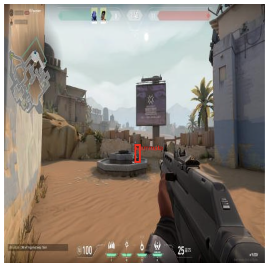
Finally, we use draw_multiple_bounding_boxes to visualize the bounding boxes and labels on the image, as shown in Figure 10.

---

Run Inference (Predicted Result)

Now, we run inference using the pre-trained PaliGemma model to detect objects in the test image. This will help us compare the model’s predictions with the ground truth.

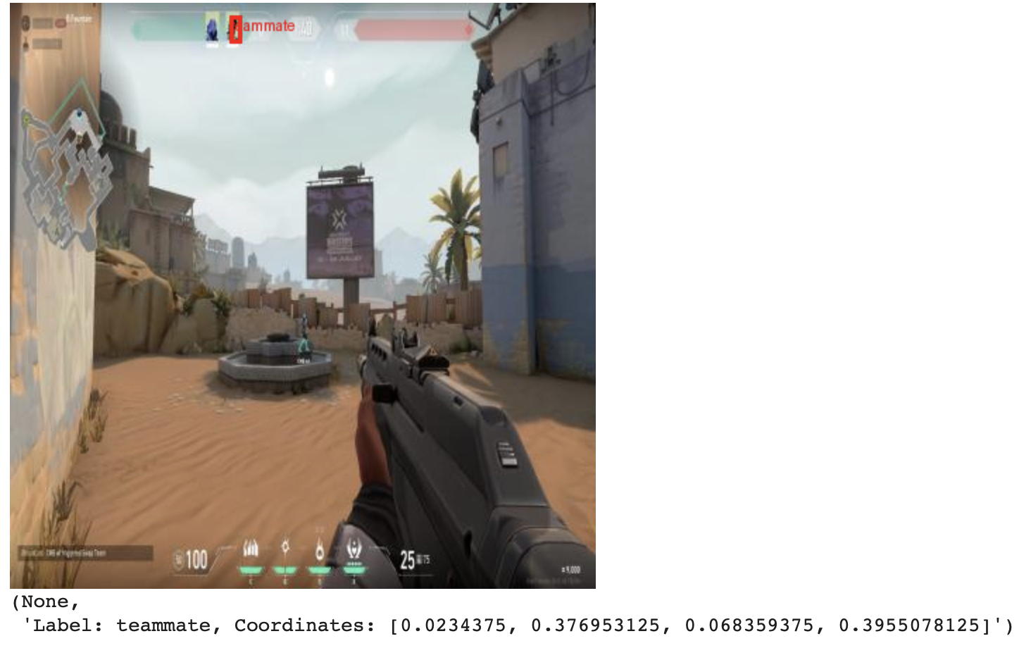
process_image(test_image, "detect teammate")

We pass the test image along with a detection prompt to the processing function (process_image).

Here, "detect teammate" acts as a prompt instructing the model to identify teammates in the image. The process_image function handles the necessary preprocessing, runs the model, and returns the predicted bounding boxes and class labels.

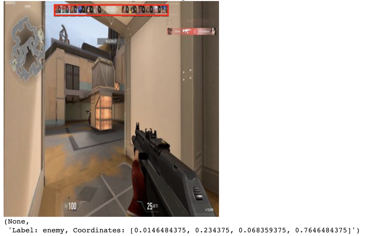
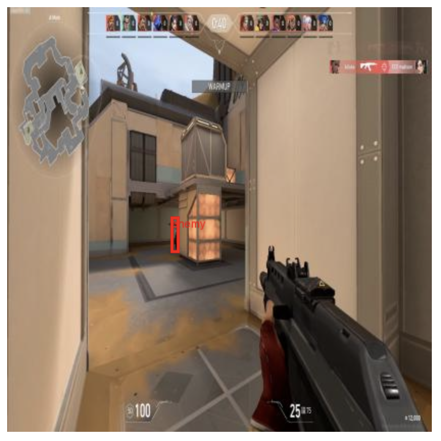
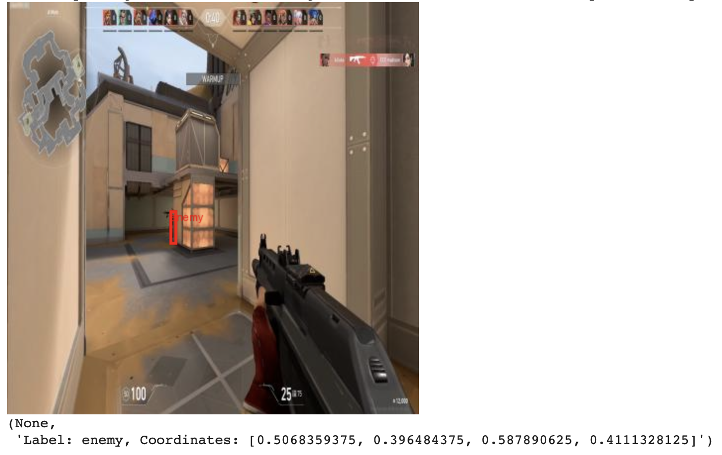
By visualizing the predicted results (Figure 11), we can see that the pre-trained model does not produce an accurate result.

---

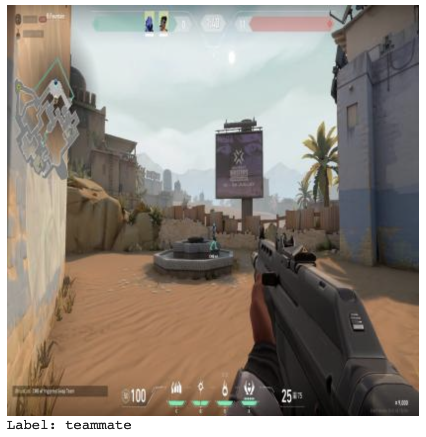
Example 2

Let’s also see one more inference output with the pre-trained PaliGemma 2 model.

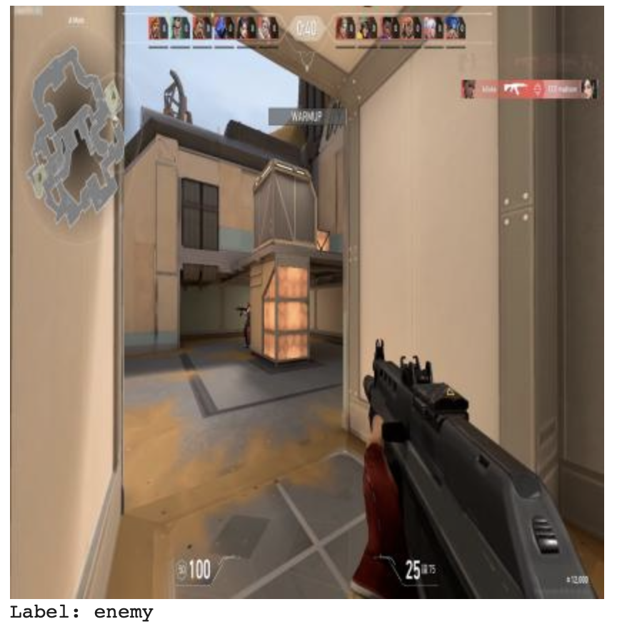
In Figure 12, we can see the new test image and the label.

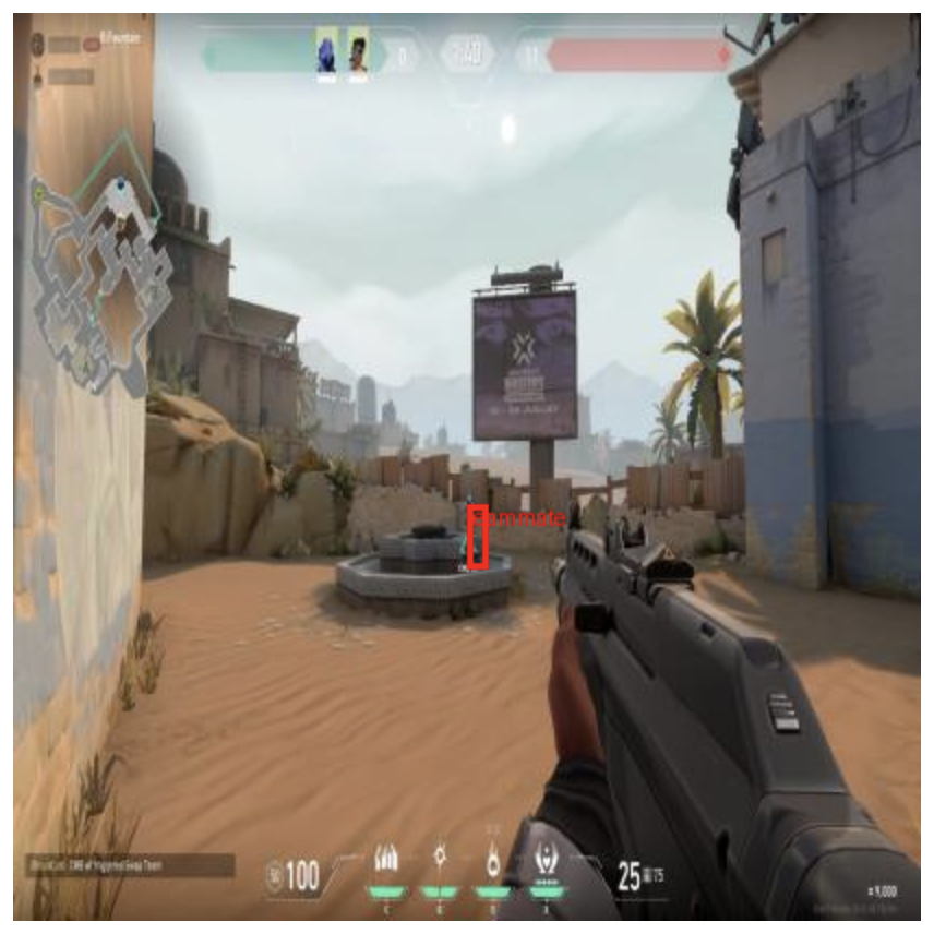
In Figure 13, we can see the Ground Truth bounding box and label.

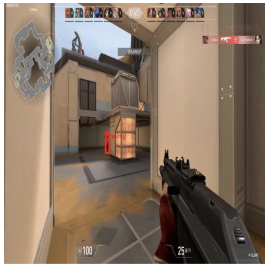
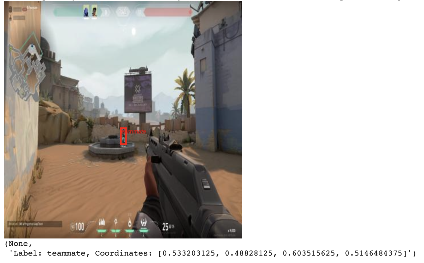
In Figure 14, we can see the predicted bounding box and label using the pre-trained PaliGemma 2 model.

We observe that the pre-trained model’s predictions are inaccurate. Therefore, we fine-tune the model on a custom dataset. After fine-tuning, we run inference again to verify whether the accuracy has improved.

We now proceed with fine-tuning the pre-trained PaliGemma 2 model using our paligemma-formatted custom dataset.

---

Fine-Tune the Model

To fine-tune the model, we will take learnings from our tutorial on Fine Tune PaliGemma with QLoRA for Visual Question Answering.

---

Load the PaliGemma-Formatted Dataset

First, let’s start with loading the PaliGemma-formatted dataset.

valorant_od_paligemma_ds = load_dataset("pyimagesearch/valorant-object-detection-paligemma")

We will use the same load_dataset function to load it.

---

Train, Validation, and Test

train_ds = valorant_od_paligemma_ds["train"]
validation_ds = valorant_od_paligemma_ds["validation"]
test_ds = valorant_od_paligemma_ds["test"]

Once loaded, we can store the dataset splits into the train_ds, validation_ds, and test_ds variables.

train_ds

In Figure 15, we can see the train dataset structure by printing train_ds. We can see all the features and the total number of examples in the training dataset.

validation_ds

In Figure 16, we can see the validation dataset structure by printing validation_ds. We can see all the features and the total number of examples in the validation dataset.

test_ds

In Figure 17, we can see the test dataset structure by printing test_ds. We can see all the features and the total number of examples in the test dataset.

---

Load the Pre-Trained PaliGemma 2 Processor

Now, let’s load the pre-trained PaliGemma 2 processor to prepare input data for the model.

device = "cuda"
pretrained_model_id = "google/paligemma2-3b-pt-224"

First, we specify the device as "cuda" to leverage GPU acceleration for faster processing. Then, we define the pre-trained model ID as "google/paligemma2-3b-pt-224", which refers to the base version of the PaliGemma 2 model.

pretrained_processor = PaliGemmaProcessor.from_pretrained(pretrained_model_id)

Finally, we initialize the PaliGemmaProcessor using the from_pretrained method.

---

Load the Pre-Trained PaliGemma 2 Model with the BitsAndBytes Configuration

To efficiently load the PaliGemma model, we use BitsAndBytesConfig for 4-bit quantization. This reduces memory consumption while maintaining performance, making it easier to run large models on limited hardware.

bnb_config = BitsAndBytesConfig(
       load_in_4bit=True,
       bnb_4bit_quant_type="nf4",
       bnb_4bit_compute_dtype=torch.bfloat16
)

First, we configure bnb_config to enable 4-bit loading by setting load_in_4bit=True. We specify "nf4" (Normalized Float 4) as the quantization type, which improves numerical stability. Additionally, we set the computation data type to torch.bfloat16, balancing precision and efficiency.

model = PaliGemmaForConditionalGeneration.from_pretrained(pretrained_model_id, quantization_config=bnb_config, device_map={"":0})

Next, we load the PaliGemmaForConditionalGeneration model using the from_pretrained() method. We pass the pre-trained model ID (pretrained_model_id) along with quantization_config=bnb_config to apply 4-bit quantization. We also set device_map={"":0} to ensure the model runs on the GPU (cuda:0).

model

Finally, we print the model to confirm that it has been successfully loaded with the specified configuration.

---

Load Model with LoRA Configuration

To fine-tune the PaliGemma model efficiently, we apply LoRA (Low-Rank Adaptation), which reduces the number of trainable parameters while maintaining performance.

lora_config = LoraConfig(
   r=8,
   target_modules=["q_proj", "o_proj", "k_proj", "v_proj", "gate_proj", "up_proj", "down_proj"],
   task_type="CAUSAL_LM",
)

First, we define lora_config using LoraConfig(). We set r=8, which controls the rank of the low-rank matrices. The target_modules list specifies which layers in the transformer (e.g., query, key, value, and projection layers) will be fine-tuned. We also set task_type="CAUSAL_LM" to indicate that this model is used for causal language modeling.

model = get_peft_model(model, lora_config)
model.print_trainable_parameters() # trainable params: 11,876,352 || all params: 3,044,118,768 || trainable%: 0.3901

Next, we apply LoRA to the pre-trained model using get_peft_model(), which wraps the loaded quantized base model with the LoRA adapters. We then print the number of trainable parameters using print_trainable_parameters(). The output confirms that only a small fraction (0.3901%) of the total model parameters are trainable, making the fine-tuning process much more efficient.

model

Finally, we print the model to verify that it has been successfully loaded with LoRA applied.

---

Preprocess the Input

Before training or inference, we need to preprocess the dataset by converting the raw inputs (images and object categories) into a format the model can understand.

category_labels = ['dropped spike', 'enemy', 'planted spike', 'teammate']
DTYPE = model.dtype

image_token = pretrained_processor.tokenizer.convert_tokens_to_ids("<image>")
def collate_fn(examples):
   texts = [f"<image>detect " + ", ".join([category_labels[int(idx)] for idx in example["objects"]["category"]]) for example in examples]
   labels= [example['paligemma_labels'] for example in examples]
   images = [example["image"].convert("RGB") for example in examples]
   tokens = pretrained_processor(text=texts, images=images, suffix=labels,
                     return_tensors="pt", padding="longest")
   tokens = tokens.to(DTYPE).to(device)
return tokens

First, we define category_labels, which maps category indices to their corresponding names: "dropped spike", "enemy", "planted spike", and "teammate". We also define the model dtype, which is torch.float16.

Next, we create a function collate_fn(examples), which processes a batch of examples. Inside the function, we generate text prompts for each example by combining <image>detect with the object categories present in the image. This ensures the model gets context about what to detect.

Then, we extract labels from paligemma_labels, which contain the bounding box information for each object. We also convert all images to RGB format to ensure consistency.

After that, we use pretrained_processor to tokenize the text prompts, process images, and append the labels as suffixes. The function returns these as tensors with padding set to "longest", ensuring all inputs in a batch have the same shape.

Finally, we move the processed tensors to torch.float16 (model DTYPE) for reduced memory usage and transfer them to the specified device (cuda for GPU acceleration). The function returns the processed batch, ready for input into the model.

---

Define Training Arguments

args=TrainingArguments(
       num_train_epochs=2,
       remove_unused_columns=False,
       per_device_train_batch_size=1,
       gradient_accumulation_steps=4,
       warmup_steps=2,
       learning_rate=2e-5,
       weight_decay=1e-6,
       adam_beta2=0.999,
       logging_steps=100,
       optim="paged_adamw_8bit",
       save_strategy="steps",
       save_steps=1000,
       save_total_limit=1,
       output_dir="pyimagesearch/valorant-od-finetuned-paligemma2",
       bf16=True,
       report_to=["tensorboard"],
       dataloader_pin_memory=False
   )

Now, let’s define the TrainingArguments to define the hyperparameters. These settings control the optimization process, checkpointing strategy, and logging.

• Epochs: We train for 2 epochs to balance performance and training time.
• Batch Size: Each device processes 1 sample per batch, with gradient accumulation steps set to 4, effectively increasing the batch size.
• Warmup Steps: We use 2 warmup steps to allow the model to adjust the learning rate gradually.
• Learning Rate and Optimizer: A learning rate of 2e-5 with AdamW (paged 8-bit variant) ensures stable convergence.
• Regularization: We apply weight decay (1e-6) to prevent overfitting and β2=0.999 for Adam optimization.
• Logging and Checkpointing: We log progress every 100 steps and save model checkpoints every 1000 steps, keeping only the latest checkpoint.
• Precision: Training runs in bfloat16 (bf16=True) for efficient mixed-precision training.
• Output Directory: The fine-tuned model is saved in "pyimagesearch/valorant-od-finetuned-paligemma2".
• Logging to TensorBoard: The training process is reported to TensorBoard for tracking metrics.

Finally, we turn off dataloader pinning (dataloader_pin_memory=False) to avoid memory issues on certain GPUs.

---

Train the Model

trainer = Trainer(
       model=model,
       train_dataset=train_ds,
       eval_dataset=validation_ds,
       data_collator=collate_fn,
       args=args
   )
trainer.train()

We use the Hugging Face Trainer API to fine-tune the PaliGemma model on the Valorant object detection dataset.

• Model: The LoRA-adapted PaliGemma model is used for training.
• Train Dataset: The train_ds dataset provides labeled examples for training.
• Validation Dataset: The validation_ds dataset is used to evaluate performance during training.
• Data Collator: The collate_fn function ensures proper tokenization and formatting of input data.
• Training Arguments: The training process follows the defined args, including batch size, learning rate, and logging settings.

Once everything is set up, we start training with: trainer.train()

This command initiates model fine-tuning, optimizing weights based on the dataset to improve object detection accuracy.

---

Push the Fine-Tuned Model to the Hugging Face Hub

trainer.push_to_hub("pyimagesearch/valorant-od-finetuned-paligemma2")

At last, we push the fine-tuned model to the Hugging Face Hub for easy access and sharing.

The fine-tuned PaliGemma model can be found here: pyimagesearch/valorant-od-finetuned-paligemma2.

---

Perform Inference with the Fine-Tuned PaliGemma Model

Once we have obtained our fine-tuned model, it’s time to put it to the test. We will now perform inference with the fine-tuned model and see if the results have improved.

---

Load the Model (Pre-Trained and Fine-Tuned)

Let’s load the pre-trained model processor and fine-tuned model.

pretrained_model_id = "google/paligemma2-3b-pt-224"
finetuned_model_id = "pyimagesearch/valorant-od-finetuned-paligemma2"

First, we define the pretrained_model_id and finetuned_model_id.

pretrained_processor = PaliGemmaProcessor.from_pretrained(pretrained_model_id)

Next, we load the pre-trained model processor using the from_pretrained method from PaliGemmaProcessor.

finetuned_model = PaliGemmaForConditionalGeneration.from_pretrained(finetuned_model_id)

Finally, we load the fine-tuned model using the from_pretrained method from PaliGemmaForConditionalGeneration.

---

Parse Multiple Locations

# Helper function to parse multiple <loc> tags and return a list of coordinate sets and labels
def parse_multiple_locations(decoded_output):
   # Regex pattern to match four <locxxxx> tags and the label at the end (e.g., 'cat')
   loc_pattern = r"<loc(\d{4})><loc(\d{4})><loc(\d{4})><loc(\d{4})>\s+([^;]+)"

   matches = re.findall(loc_pattern, decoded_output)
   coords_and_labels = []

   for match in matches:
       # Extract the coordinates and label
       y1 = int(match[0]) / 1024
       x1 = int(match[1]) / 1024
       y2 = int(match[2]) / 1024
       x2 = int(match[3]) / 1024
       label = match[4].strip()

       coords_and_labels.append({
           'label': label,
           'bbox': [y1, x1, y2, x2]
       })

   return coords_and_labels

To parse multiple <loc> tags and return a list of coordinate sets and labels, we use the same parse_multiple_locations function as we defined before.

---

Draw Multiple Bounding Boxes

# Helper function to draw bounding boxes and labels for all objects on the image
def draw_multiple_bounding_boxes(image, coords_and_labels):
   draw = ImageDraw.Draw(image)
   width, height = image.size

   for obj in coords_and_labels:
       # Extract the bounding box coordinates
       y1, x1, y2, x2 = obj['bbox'][0] * height, obj['bbox'][1] * width, obj['bbox'][2] * height, obj['bbox'][3] * width

       # Draw bounding box and label
       draw.rectangle([x1, y1, x2, y2], outline="red", width=3)
       draw.text((x1, y1), obj['label'], fill="red")

   return image

To draw bounding boxes and labels for all objects on the image, we define the same draw_multiple_bounding_boxes as we defined before.

---

Define Inference Function

# Define inference function
def process_image(image, prompt):
   # Process the image and prompt using the processor
   inputs = pretrained_processor(image.convert("RGB"), prompt, return_tensors="pt")

   try:
       # Generate output from the model
       output = finetuned_model.generate(**inputs, max_new_tokens=100)

       # Decode the output from the model
       decoded_output = pretrained_processor.decode(output[0], skip_special_tokens=True)

       # Extract bounding box coordinates and labels
       coords_and_labels = parse_multiple_locations(decoded_output)

       if coords_and_labels:
           # Draw bounding boxes and labels on the image
           image_with_boxes = draw_multiple_bounding_boxes(image, coords_and_labels)

           # Prepare the coordinates and labels for the UI
           labels_and_coords = "\n".join([f"Label: {obj['label']}, Coordinates: {obj['bbox']}" for obj in coords_and_labels])

           # Return the modified image and the list of coordinates+labels
           return display(image_with_boxes), labels_and_coords
       else:
           return "No bounding boxes detected."

   except IndexError as e:
       print(f"IndexError: {e}")
       return "An error occurred during processing."

We defined the same inference process_image function as before to process an image and a text prompt, extract bounding box information, and return an annotated image with object labels. The only difference is the use of finetuned_model to generate the response instead of pretrained_model.

---

Example 1

Now, let’s see whether the fine-tuned model has improved the result. We will take the same examples as before to compare the results.

---

Display Test Image and Label

# Get the first example from the test dataset
test_example = valorant_od_paligemma_ds["test"][0]

# Extract the image and objects
test_image = test_example["image"]
categories_idx = test_example["objects"]["category"]  # List of category indices
category_labels = ['dropped spike', 'enemy', 'planted spike', 'teammate']  # Example category names

# Display the image
display(test_image)

# Display the category names for each object in the image
for idx in categories_idx:
   category_name = category_labels[idx]  # Map the index to the label name
   print(f"Label: {category_name}")

Let’s display the test image and label again by taking the first example from the test dataset as before.

In Figure 18, we can see the test image and the label.

---

Ground Truth

Let’s examine the ground truth bounding box and label again to verify the dataset annotations and compare them later with the model’s predictions.

test_coords_and_labels = valorant_od_paligemma_ds["test"][0]["paligemma_labels"]

coords_and_labels = parse_multiple_locations(test_coords_and_labels)
coords_and_labels

The steps to get the ground truth remain the same.

In Figure 19, we can see label and a list of bounding box coordinates.

draw_multiple_bounding_boxes(test_image, coords_and_labels)

In Figure 20, we can visualize the bounding box and label on the image.

---

Run Inference (Predicted Result)

Finally, we run inference using the fine-tuned PaliGemma 2 model to detect objects in the test image. This will help us compare the model’s predictions with the ground truth.

process_image(test_image, "detect teammate")

We can see (Figure 21) that the fine-tuned model produced an accurate result that matches the ground truth.

Hence, after fine-tuning the base pre-trained PaliGemma model, the model can be adapted to detecting objects in the Valorant game.

---

Example 2

Let’s also see one more inference output with the fine-tuned PaliGemma 2 model.

In Figure 22, we can see the test image and the label.

In Figure 23, we can see the ground truth bounding box and label.

In Figure 24, we can see the predicted bounding box and label using the fine-tuned PaliGemma 2 model.

From these two examples, it is evident that fine-tuning the model has clearly improved the results in detecting objects in the Valorant game.

---

Summary

In this tutorial, we fine-tuned the PaliGemma 2 model to detect objects in Valorant using a custom-formatted dataset. We first evaluated the pre-trained model’s performance, which proved inaccurate for this task. Then, we processed the dataset, applied LoRA-based fine-tuning, and optimized training with BitsAndBytes quantization. After training, the fine-tuned model showed improved detection accuracy, demonstrating the effectiveness of task-specific adaptation. This approach can be extended to other object detection tasks in gaming and beyond.

In an upcoming tutorial, we will explore how a fine-tuned model can detect brain tumors in medical images. Watch for updates!

---

Citation Information

Thakur, P. “Object Detection in Gaming: Fine-Tuning Google’s PaliGemma 2 for Valorant,” PyImageSearch, P. Chugh, S. Huot, and G. Kudriavtsev, eds., 2025, https://pyimg.co/sx8l4

@incollection{Thakur_2025_object-detection-gaming-fine-tuning-googles-paligemma-2-valorant,
  author = {Piyush Thakur},
  title = {{Object Detection in Gaming: Fine-Tuning Google's PaliGemma 2 for Valorant}},
  booktitle = {PyImageSearch},
  editor = {Puneet Chugh and Susan Huot and Georgii Kudriavtsev},
  year = {2025},
  url = {https://pyimg.co/sx8l4},
}

---

To download the source code to this post (and be notified when future tutorials are published here on PyImageSearch), simply enter your email address in the form below!