Implementing Semantic Search: Jaccard Similarity and Vector Space Models

---

Table of Contents

---

Implementing Semantic Search: Jaccard Similarity and Vector Space Models

In this tutorial, you will learn the mechanisms and mathematical and computational models that power semantic search. We will start by understanding the limitations of Boolean search models and then learn:

• How documents and queries can be represented as vectors
• How scoring techniques can be used to compute query-document relevance

As a hands-on, we will implement TF-IDF and Sentence-BERT based semantic search models in Python.

This lesson is the 2nd of a 3-part series on Unlocking the Power of Search: Boolean, Semantic, and Probabilistic Search Models Explained.

1. Boolean Search: Harnessing AND, OR, and NOT Gates with Inverted Indexes
2. Implementing Semantic Search: Jaccard Similarity and Vector Space Models (this tutorial)
3. Exploring Probabilistic Search: The Power of the BM25 Algorithm

To learn how Semantic Search works, just keep reading.

---

Implementing Semantic Search: Jaccard Similarity and Vector Space Models

---

Beyond Boolean Search: Navigating Limitations and Opportunities

In a previous lesson, we learned how an inverted index can be used to construct a Boolean search model that is capable of retrieving relevant documents based on a Boolean query. However, there are several things to keep in mind while using Boolean queries or Boolean search models:

• No Ranking: Documents either match or do not. Boolean search can’t retrieve documents that are partially relevant to the query. There is no way to compare the relevance of documents retrieved by a Boolean search model. A Boolean search can result in 1000s of retrieved documents, however most users don’t want to wade through 1000s of results.
• Boolean Queries: Most users are incapable of writing Boolean queries (or they are, but they think it’s too much work). Boolean queries are apt for users who have a precise and objective understanding of their needs and the collection. If one precisely knows what they are looking for, then using a Boolean search model becomes very easy.
• Feast or Famine: Boolean queries often result in either too few (when there are too many AND operations) or too many (if there are many OR operations) results. Hence, it takes a lot of skill to come up with a query that produces a manageable number of hits.

Thus, rather than a set of documents satisfying a query expression (e.g., in a Boolean search), we need a system that can rank documents in order of their relevance to the query. Ranked retrieval exactly addresses the above requirements. In ranked retrieval, the system returns an order over the (top) documents in the collection for a query.

In ranked retrieval, even when the system produces a large set of relevant documents, it’s not a problem! In such a case, we can show the top K (e.g., 10, 20) results based on their ranks (relevance to the query).

Further, rather than specifying a query in terms of operators and operands, the system should support queries that are simple to construct and interpret (e.g., natural language). Ranked retrieval is normally associated with such free text queries.

Figure 1 illustrates the difference between a Boolean search and a semantic search model.

---

Scoring: A Deep Dive into Jaccard Similarity for Retrieval

As we just learned, in ranked retrieval, we wish to return in order the documents most likely to be useful to the user. But how can we achieve that? How can we rank the documents in the collection with respect to the query?

The idea is to assign a score — say in [0,1] — to each document that measures how relevant the document is for the query. A higher score (e.g., 0.9, 0.95, 0.85) indicates that the document is highly relevant to the query, while a lower score (e.g., 0.1, 0.05, etc.) indicates that the document is irrelevant to the query.

A very common and popular approach to scoring documents based on a query is known as the Jaccard coefficient or Jaccard similarity score. The Jaccard similarity score (Figure 2) treats documents and queries as sets of terms and computes the overlap between these sets.

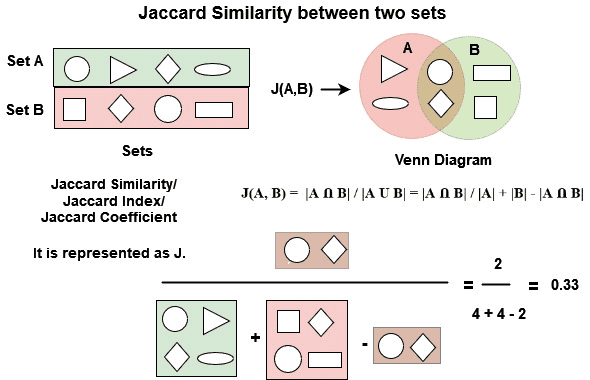
To understand better, suppose a document and query are represented as a set of terms that consist of:

Jaccard similarity then computes the overlap between these two sets and as:

This way, the Jaccard similarity score always assigns a number between 0 and 1, which indicates how similar the document and query sets are. Further, with Jaccard similarity, the document and query sets don’t have to be the same size.

As an example, consider the following:

• Q: machine learning projects
• Document D1: top machine learning projects for beginners
• Document D2: how machine translation works

The set representation of query and documents are:

• 
• 
• 

The Jaccard similarity will be as follows:

• 
• 

Since , this indicates that document is more relevant than for query .

---

Vector Space Models: The Power of TF-IDF Weighting

Do you see any issues with the Jaccard similarity score?

• Term Frequency: The Jaccard similarity score doesn’t consider term frequency (how many times a term occurs in a document). More often, rare terms in a collection are more informative than frequent terms. Jaccard doesn’t consider this information.
• Document Length Normalization: Secondly, the Jaccard similarity score doesn’t take document length normalization into account. Imagine a document containing 1000s of terms, but the query is only 2-3 terms. The Jaccard coefficient will return a score in the order of 1e-3.

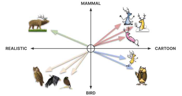
To address these issues, we will now move toward vector space models (semantic search models). These models or algorithms consider documents and queries as -dimensional vectors (Figure 3) rather than variable length sets (as in Jaccard similarity). By considering them as fixed-dimensional vectors, we remove the dependence on document length as each document, no matter how long, will be represented by a fixed-dimensional vector.

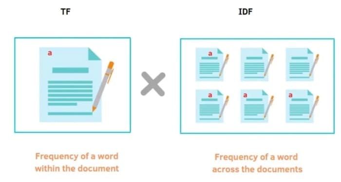
We will start with our first semantic search algorithm (i.e., TF-IDF weighting). TF-IDF, which stands for Term Frequency-Inverse Document Frequency, is a statistical measure used in information retrieval and text mining to evaluate the importance of a word in a document relative to a collection of documents (or corpus).

TF-IDF based semantic search represents documents and queries as fixed-dimensional vectors, where each dimension corresponds to a term in the vocabulary, and the value represents its importance in a document relative to a collection of documents.

Let’s start by understanding the components of TF-IDF weighting (i.e., Term Frequency (TF) and Inverse Document Frequency (IDF)).

---

Understanding the Importance of Term Frequency

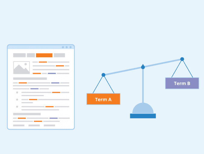
Term frequency (Figure 4) measures how frequently a term appears in a document. The idea of Term Frequency is that a document with 10 occurrences of the term is more relevant than a document with one occurrence of the same term.

The term frequency of term in document is defined as the number of times that occurs in

However, there is one small issue with using term frequency to evaluate the importance of a word in a document. If document has 10 occurrences of the term, that does not indicate that is 10 times more relevant than .

In other words, the relevance of a word in a document does not increase proportionally with term frequency. Hence, we use log-frequency () of the term in document :

---

Unlocking Inverse Document Frequency for Enhanced Retrieval

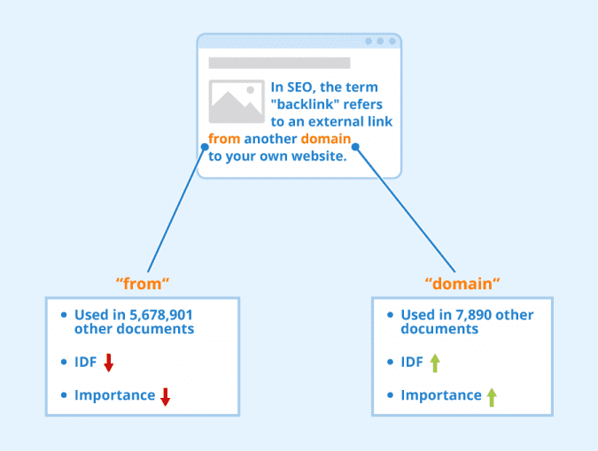
Rare terms are more informative than frequent terms. For example, stop words (i.e., “a,” “an,” “the,” and “is”) are usually quite-frequent terms in a collection. However, such terms are not very meaningful. This implies that the term frequency alone is not sufficient to measure the importance of a term in a document or collection.

Consider a term in the query that is rare in the collection (e.g., arachnocentric). A document containing this term is very likely to be relevant to the query “arachnocentric,” and hence, we want a high weight for rare terms like “arachnocentric.”

Inverse Document Frequency (IDF) (Figure 5) addresses exactly this. Inverse document frequency is defined as the logarithm of the inverse of document frequency.

where is the document frequency (i.e., the number of documents that contain the term ). In simpler words, is an inverse measure of the informativeness of the term .

Note that we use instead of to “dampen” the effect of .

---

TF-IDF Weighting

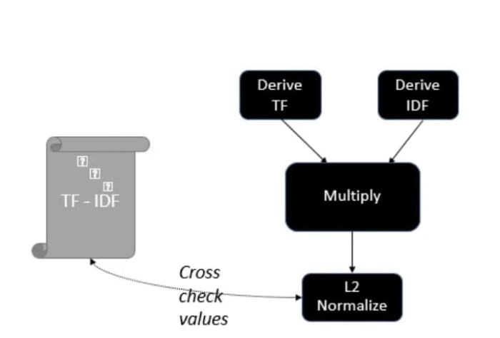
The TF-IDF weight (Figure 6) of a term is the product of its TF (term frequency) weight and its IDF (inverse document frequency) weight.

TF-IDF weighting is one of the best-known weighting schemes in information retrieval. The weighting scheme takes both things into account:

• Increases with the number of occurrences of a term within a document.
• Increases with the rarity of the term in the collection.

With TF-IDF weighting, we can now represent our documents and queries as vectors. Suppose we have terms in the vocabulary, then each document and query vector:

• Will be a -dimensional vector.
• Terms are axes of the space and the value of these axes will be the TF-IDF weight of each term.

---

Cosine Similarity for Measuring Semantic Proximity

Now that we have a -dimensional vector representation of document and query , we need a proximity measure (Figure 7) that can tell us how similar these two vectors are in the vector space. The more similar the query-document vectors are, the more relevant the document is to the query.

One way to measure the proximity of two vectors in a vector space is to consider the inverse of the Euclidean distance between the two vectors:

The more the distance between the vectors, the lesser the similarity between them. However, there is one issue with using Euclidean distances for proximity measures. Can you guess what?

Consider a thought experiment where you take a document and append it to itself. Let’s call this document . “Semantically” and have the same content. However, the Euclidean distance between the two documents can be quite large!

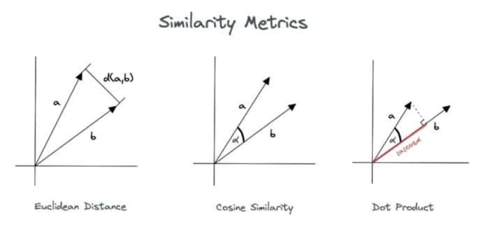
Thus, the Euclidean distance (Figure 8) is large for vectors of different lengths and doesn’t provide an appropriate measure. Then what else can we do?

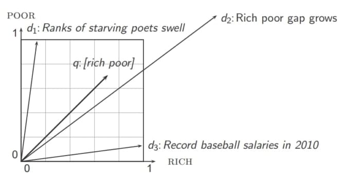
Well, in the above thought experiment, if you noticed, the “angle” between the two documents and is 0, corresponding to the maximal similarity. Hence, the key idea is to rank documents according to the angle with the query. The lesser the angle between the document and query vector, the more the similarity between them!

The following two notions are equivalent.

• Rank documents in decreasing order of the angle between query and document, OR
• Rank documents in increasing order of (as cosine is a monotonically decreasing function for the interval ).

Figure 9 explains the difference between different similarity measures. Both cosine similarity and dot product are equivalent terms.

The cosine similarity (Figure 10) score between a document and a query vector is defined as the dot product between the document-query unit vectors:

where denotes the dot product between two vectors and .

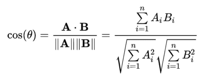
As you have noticed, cosine similarity normalizes the documents by their Euclidean norm , which means that document/query length doesn’t play any role in the similarity between both vectors. This makes cosine similarity measure an apt and widely-opted choice for computing similarity in vector space models.

---

How to Build a TF-IDF-Based Semantic Search for ArXiv Paper Abstracts

Now, let’s learn to implement a Semantic search model on the arXiv paper abstract dataset. The arXiv paper dataset consists of 50K+ paper titles and abstracts from various research areas.

The goal is to build a model that can retrieve relevant ArXiv papers for a given free text query, such as: “machine learning for covid-19 using GANs.”

---

Step-by-Step Guide to Downloading the ArXiv Paper Abstract Dataset

We will download our arXiv paper abstract dataset using the Kaggle API. Here’s how you can install the Kaggle API and the arXiv dataset on your system:

$ pip install kaggle
$ kaggle datasets download -d spsayakpaul/arxiv-paper-abstracts
$ unzip <path-to-zip>/arxiv-paper-abstracts.zip -d /<path-to-data>/

---

Loading and Preparing the ArXiv Dataset for Analysis

Before loading our arXiv paper abstract dataset, let’s install some important Python libraries that we will use in this project:

• nltk: The Natural Language Toolkit (NLTK) is a comprehensive Python library that provides a suite of tools for tasks such as tokenization, stemming, lemmatization, part-of-speech tagging, and named entity recognition.
• scikit-learn (sklearn): Scikit-learn is a free and open-source machine learning library for the Python programming language. It features various classification, regression, and clustering algorithms (e.g., support vector machines, TF-IDF models, neural networks, etc.).
• pandas: Pandas is a powerful, open-source Python library for data manipulation and analysis. We will use pandas to read and manipulate our datasets saved in CSV format.
• numpy: NumPy is a popular Python library that supports large, multi-dimensional arrays and matrices, along with a large collection of high-level mathematical functions.

Here’s how to install the required Python libraries using pip.

$ pip install pandas numpy nltk scikit-learn

Next, we will import these libraries into our Jupyter Notebook and load and visualize the dataset.

!pip install contractions
import numpy as np
import pandas as pd
from nltk.stem import PorterStemmer
from nltk.corpus import stopwords
import sklearn
import nltk

nltk.download('stopwords')

from IPython.display import display, HTML

data = pd.read_csv("/<path-to-data>/arxiv_data.csv", header='infer')
print("Total rows : ", len(data))

display(HTML(data.head().to_html()))

On Lines 1-7, we import the pandas, numpy, nltk, and sklearn libraries. Next, on Line 9, we download the list of stopwords from the nltk package.

On Lines 13-16, we load the arxiv_data.csv using the pandas.read_csv() utility. We print the number of rows in the dataset and also visualize some of them using the IPython display. Figure 11 displays the output of the above code block.

Each row in the dataset has three fields:

• titles: The title of the research paper.
• summaries: The abstract of the research paper.
• terms: The tags associated with the paper.

---

Constructing a TF-IDF Index Using Sklearn

Next, we will construct a TF-IDF index over the whole corpus of ArXiv abstracts. Using sklearn.feature_extraction.text.TfidfVectorizer, we can convert all documents as well as queries to a fixed-length TF-IDF vector.

Instead of considering all terms in the vocabulary (> 50000), we will only choose the top 5000 terms from the corpus and build a TF-IDF index based on them. This means that each document and query vector will be 5000 in size.

The value of each element in the vector will be the TF-IDF based on the corresponding term in the document (paper abstracts in our case).

from sklearn.feature_extraction.text import TfidfVectorizer

stemmer = PorterStemmer()
stop_words = set(stopwords.words("english"))


corpus = []

for summary in data.summaries.to_list():
  tokens = summary.lower().split()
  # Stemming and stop-word removal
  tokens = [stemmer.stem(token) for token in tokens if token not in stop_words]
  corpus.append(" ".join(tokens))

print(corpus[0])

# create a TF-IDF index based on the whole corpus
vectorizer = TfidfVectorizer(sublinear_tf=True, max_features=5000)
vectorizer.fit_transform(corpus)

# Print features used for TF-IDF vectorization
print("Total features ", vectorizer.get_feature_names_out().shape)
vectorizer.get_feature_names_out()[:1000]

Let’s understand the above code snippet line-by-line.

On Line 17, we begin by importing the sklearn.feature_extraction.text.TfidfVectorizer class, which converts a collection of raw text documents into a matrix of TF-IDF (Term Frequency-Inverse Document Frequency) features.

On Lines 19-29, we perform basic preprocessing steps on the arXiv abstracts. For each summary in the data.summaries list, we split the summary into lowercase tokens (words). After that, we apply stemming and stop-word removal where each token is stemmed (reduced to its root form) using the Porter stemmer, and stop words (common words like “the,” “and,” etc.) are removed. The processed tokens are joined back into a single string and added to the corpus.

On Line 34, we create an instance vectorizer of TfidfVectorizer with:

• sublinear_tf=True: Applies a sublinear (log-frequency) scaling to the term frequency (TF) values.
• max_features=5000: Limits the number of features (unique words) to 5000.
• Other default settings are used for parameters like analyzer, lowercase, etc.

On Line 35, the vectorizer is fitted to the corpus using the fit_transform method. This step calculates the TF-IDF values for each term in the corpus.

Finally, on Lines 38 and 39, we print the total number of features (unique terms) used for TF-IDF vectorization and visualize the first 1000 feature names (terms).

---

Performing a Semantic Search on a Sample Query

So far, we have processed our text data and created a TF-IDF index that stores the TF-IDF features of each term in the corpus. Now, we will show how to perform a semantic search for a sample query using this TF-IDF index.

To perform a semantic search on the corpus, we will first convert all the documents (abstracts) and the given query to their TF-IDF vector representations. Once we have the vector representations of all the documents, we will compute their cosine similarity with the query vector, and pick the TopK document indices with the highest cosine similarity.

from sklearn.metrics.pairwise import cosine_similarity

# Converting documents to their fixed length feature vector
documents_tfidf_features = vectorizer.transform(corpus)

TopK = 10

# sample query
query = "machine learning for covid-19 research using GANs"

# query TF-IDF vector
query_tfidf_features = vectorizer.transform([query])
print("TF-IDF features for query", query_tfidf_features, "\n")

# Computing the cosine similarities
similarities = cosine_similarity(documents_tfidf_features, query_tfidf_features)

top_indices = similarities[:, 0].argsort()[::-1][:TopK] # Pick TopK document ids having highest cosine similarity

# Display the relevant documents
titles = []
abstracts = []
similarity = []
for doc_index in top_indices:
  titles.append(data.iloc[doc_index].titles)
  abstracts.append(data.iloc[doc_index].summaries.replace("\n", " "))

results = pd.DataFrame({"Title": titles, "Abstract": abstracts, "Similarities": similarities[top_indices, 0]} )
display(HTML(results.to_html()))

Let’s understand the above code snippet line-by-line:

On Line 43, we begin by using the vectorizer to transform a collection of pre-processed abstracts (referred to as “corpus”) into fixed-length feature vectors using the Term Frequency-Inverse Document Frequency (TF-IDF) representation. We also define the TopK variable that specifies the number of relevant documents to retrieve.

On Lines 48-55, we define a sample query sample query: "machine learning for covid-19 using GANs". The query is transformed into a TF-IDF vector using the same vectorizer.

Once we have the query vector, we compute the cosine similarity between the query vector and all document vectors using sklearn.metrics.pairwise.cosine_similarity. Cosine similarity measures the angle between two vectors and ranges from -1 (completely dissimilar) to 1 (identical). The similarities array contains the cosine similarity scores for each document with respect to the query.

On Lines 57-68, we identify the indices of the top-K documents (highest cosine similarity scores) based on the similarities array. Then, for each relevant document, the title and abstract are extracted from the original dataset (data) using the corresponding indices. The results are displayed in a Pandas DataFrame, including columns for the title, abstract, and similarity score.

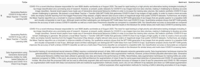
Figure 12 displays the result of the above code snippet.

As you can see from the output, for our sample query, "machine learning for covid-19 using GANs", the TF-IDF based semantic search can retrieve and rank documents based on their relevance.

---

Harnessing Embeddings for Semantic Search

As we just saw, TF-IDF is able to rank documents based on their relevance to the query, which is a much superior feature to a Boolean search model. However, there are several things to keep in mind while using TF-IDF based semantic search:

• Polysemy: Their TF-IDF weighting only considers the frequency of terms and does not understand their meaning or context. This can sometimes lead to irrelevant results, even when the same word can have different meanings in different contexts.
  
  For example, consider the word “bank”:
  1. “I need to go to the bank to deposit some money.”
  2. “We had a picnic on the bank of the river.”
  
  In a TF-IDF-based search, both sentences would be treated similarly because they contain the word “bank.” However, the context is entirely different. TF-IDF does not understand that “bank” refers to a financial institution in the first sentence and a riverbank in the second.

• Synonyms: Further, TF-IDF cannot recognize synonyms or related terms. As an example, “car” and “automobile” are synonyms but will be treated as completely different terms in TF-IDF weighting.

This is where embedding-based semantic search comes into play, offering a more nuanced and effective approach.

Embedding-based semantic search leverages advanced machine learning models to transform documents and queries into their corresponding vector representations, known as embeddings. These embeddings capture the semantic meaning of the text, allowing the search engine to understand and retrieve information based on context rather than just keyword matching.

Often, these embeddings are generated using neural network models (Figure 13), such as BERT (Bidirectional Encoder Representations from Transformers) or GPT (Generative Pre-trained Transformer). These models are trained on vast amounts of text data to understand language patterns and relationships.

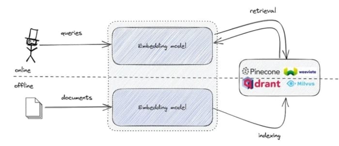
Embedding-based search can understand synonyms and related concepts. For example, a search for “running shoes” will also retrieve results for “sneakers”. Furthermore, they are less sensitive to exact phrasing, spelling mistakes, and grammatical errors, making them more robust to variations in how queries are phrased.

In an embedding-based semantic search, documents and queries are embedded into a vector space. Each dimension in this space captures different aspects of the text’s meaning. Then, similar to a TF-IDF semantic search, we compute the cosine similarity between the document and query embeddings to rank the document.

---

Step-by-Step Guide to Building an Embedding-Based Semantic Search Engine for ArXiv Abstracts

In this section, we will implement an embedding-based similar semantic search model using Sentence-Transformers.

---

Loading Our Sentence-Transformer Model

Sentence Transformers (a.k.a. SBERT) is the go-to Python module for accessing, using, and training more than 5000 state-of-the-art text and image embedding models.

We will first install the sentence-transformers library. Here’s how to install it using pip.

$ pip install sentence-transformers

Next, we will load our Sentence Transformer in CUDA memory.

from sentence_transformers import SentenceTransformer

# 1. Load a pretrained Sentence Transformer model
model = SentenceTransformer("all-MiniLM-L6-v2", device="cuda")

Note: To ensure the model utilizes GPU runtime, connect your Colab notebook to a GPU runtime.

Here, we load all-MiniLM-L6-v2, which is a sentence-transformers model. It maps sentences and paragraphs to a 384-dimensional dense vector space and can be used for tasks like clustering or semantic search.

The model is fine-tuned on a 1B sentence pairs dataset using a contrastive learning objective. Given a sentence from the pair, the model should predict which, out of a set of randomly sampled other sentences, was actually paired with it in our dataset.

---

Performing Embedding-Based Semantic Search on a Sample Query

Similar to TF-IDF based semantic search, we will now use the loaded sentence transformer model to obtain the vector representations (a.k.a. embeddings) for each document and the query.

Once we have the embeddings of all the documents, we will compute their cosine similarity with the query embedding and pick the TopK document indices with the highest cosine similarity.

TopK = 10

# Computing the embeddings of documents
passage_embeddings = model.encode(corpus)
print(passage_embeddings.shape)

# compute query embedding
query_embedding = model.encode("machine learning for covid-19 research using GANs")
similarities = model.similarity(query_embedding, passage_embeddings).numpy() # cosine similarities

top_indices = similarities[0, :].argsort()[::-1][:TopK] # pick TopK documents having highest cosine similarity

# Display the documents
titles = []
abstracts = []
similarity = []
for doc_index in top_indices:
  titles.append(data.iloc[doc_index].titles)
  abstracts.append(data.iloc[doc_index].summaries.replace("\n", " "))

results = pd.DataFrame({"Title": titles, "Abstract": abstracts, "Similarities": similarities[0, top_indices]} )
display(HTML(results.to_html()))

Let’s understand the above code snippet line-by-line.

On Lines 73-77, we begin by defining the TopK variable that specifies the number of relevant documents to retrieve. Then, we use the model.encode function to compute the fixed-dimensional embeddings of pre-processed abstracts (referred to as “corpus”). These embeddings are referred to as passage_embeddings.

On Lines 80 and 81, we compute the embedding vector for a sample query and compute the cosine similarity between the query embedding and all passage embeddings using model.similarity.

On Lines 83-94, we identify the indices of the top-K documents (highest cosine similarity scores) based on the similarities array. Then, for each relevant document, the title and abstract are extracted from the original dataset (data) using the corresponding indices. The results are displayed in a Pandas DataFrame, including columns for the title, abstract, and similarity score.

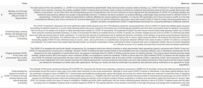
Figure 14 displays the result of the above code snippet.

From the output, we can see that for the same sample query, the embedding-based semantic search is able to retrieve more relevant documents compared to the TF-IDF based semantic search. As you have observed, the cosine similarities between the document and the query are also much higher compared to the TF-IDF based semantic search.

This explains that embedding-based semantic search allows the search engine to understand and retrieve information based on context rather than just keyword matching.

---

---

Summary

In the blog post, We first delve into the concept of implementing semantic search using Jaccard Similarity and Vector Space Models, moving beyond the limitations and opportunities of Boolean Search. We take a deep dive into the scoring mechanism, particularly focusing on the use of Jaccard Similarity for retrieval. This sets the stage for the introduction of Vector Space Models and the power of TF-IDF (Term Frequency-Inverse Document Frequency) weighting.

We then explore the importance of Term Frequency and how it plays a crucial role in understanding the relevance of a term in a document. This is followed by an explanation of Inverse Document Frequency and how it can be unlocked for enhanced retrieval. We discuss TF-IDF weighting in detail, explaining how it combines the concepts of term frequency and inverse document frequency to assign a weight to each term in a document.

Next, we introduce the concept of Cosine Similarity for measuring semantic proximity, which is a critical component in semantic search. We provide a practical guide on how to build a TF-IDF based semantic search for ArXiv Paper Abstracts. This includes a step-by-step guide to downloading the ArXiv Paper Abstract Dataset, loading and preparing the dataset for analysis, and constructing a TF-IDF index using Sklearn.

Finally, We discuss the concept of harnessing embeddings for semantic search by providing a detailed guide on building an embedding-based semantic search engine for ArXiv Abstracts. This involves loading our Sentence-Transformer model and performing an embedding-based semantic search on a sample query. The blog post is a comprehensive guide that combines theory with practical implementation, providing readers with a deep understanding of semantic search and its applications.

---

Citation Information

Mangla, P. “Implementing Semantic Search: Jaccard Similarity and Vector Space Models,” PyImageSearch, P. Chugh, A. R. Gosthipaty, S. Huot, K. Kidriavsteva, and R. Raha, eds., 2024, https://pyimg.co/9bzn2

@incollection{Mangla_2024_Implementing-Semantic-Search,
  author = {Puneet Mangla},
  title = {Implementing Semantic Search: Jaccard Similarity and Vector Space Models},
  booktitle = {PyImageSearch},
  editor = {Puneet Chugh and Aritra Roy Gosthipaty and Susan Huot and Kseniia Kidriavsteva and Ritwik Raha},
  year = {2024},
  url = {https://pyimg.co/9bzn2},
}