What’s New in PyTorch 2.0? torch.compile

---

Table of Contents

---

What’s New in PyTorch 2.0? torch.compile

Over the last few years, PyTorch has evolved as a popular and widely used framework for training deep neural networks (DNNs). The success of PyTorch is attributed to its simplicity, first-class Python integration, and imperative style of programming. Since the launch of PyTorch in 2017, it has strived for high performance and eager execution. It has provided some of the best abstractions for distributed training, data loading, and automatic differentiation.

With continuous innovation from the PyTorch team, PyTorch has moved from version 1.0 to the most recent version, 1.13. However, over all these years, hardware accelerators like GPUs have become 15x and 2x faster in compute and memory access, respectively. Thus, to leverage these resources and deliver high-performance eager execution, the team moved substantial parts of PyTorch internals to C++.

On December 2, 2022, the team announced the launch of PyTorch 2.0, a next-generation release that will make training deep neural networks much faster and support dynamic shapes. The stable release of PyTorch 2.0 is planned for March 2023. This blog series aims to understand and test the capabilities of PyTorch 2.0 via its beta release.

In this series, you will learn about Accelerating Deep Learning Models with PyTorch 2.0.

This lesson is the 1st of a 2-part series on Accelerating Deep Learning Models with PyTorch 2.0:

1. What’s New in PyTorch 2.0? torch.compile (today’s tutorial)
2. What’s Behind PyTorch 2.0? TorchDynamo and TorchInductor (primarily for developers)

To learn what’s new in PyTorch 2.0, just keep reading.

---

What’s New in PyTorch 2.0? torch.compile

We start this lesson by learning to install PyTorch 2.0.

---

Configuring Your Development Environment

---

Installation

Like previous versions, PyTorch 2.0 is available as a Python pip package. However, to successfully install PyTorch 2.0, your system should have installed the latest CUDA (Compute Unified Device Architecture) versions (11.6 and 11.7). Here’s how you can install the PyTorch 2.0 nightly version via pip:

For CUDA version 11.7

$ pip3 install numpy --pre torch --force-reinstall --extra-index-url https://download.pytorch.org/whl/nightly/cu117

For CUDA version 11.6

$ pip3 install numpy --pre torch --force-reinstall --extra-index-url https://download.pytorch.org/whl/nightly/cu116

However, if you don’t have CUDA 11.6 or 11.7 installed on your system, you can download all the required dependencies in the PyTorch nightly binaries with docker.

$ sudo apt install -y nvidia-docker2
$ sudo systemctl restart docker
$ docker pull ghcr.io/pytorch/pytorch-nightly
$ docker run --gpus all -it ghcr.io/pytorch/pytorch-nightly:latest /bin/bash

Be sure to specify --gpus all so that your container can access all your GPUs.

---

Verification

Optionally, you can verify your installation via:

$ git clone https://github.com/pytorch/pytorch
$ cd tools/dynamo
$ python verify_dynamo.py

---

Overview of PyTorch 2.0

Before understanding what’s new in PyTorch 2.0, let us first understand the fundamental difference between eager and graph executions (Figure 1).

Eager Execution: An eager execution evaluates the operations immediately and at run time. The programs are generally easy to write, test, and debug with a natural Python-like syntax design. However, because of its nature, it fails to fully leverage the capabilities of hardware accelerators like GPUs. PyTorch is a common example that follows eager execution.

Graph Execution: Graph execution, on the other hand, builds a graph of all operations and operands before running. Such an execution is much faster than an eager one, as the graph formed can be optimized to leverage the capabilities of hardware accelerators. However, such programs take more work to write and debug. TensorFlow is a typical example that follows graph execution.

PyTorch has always strived for high performance and eager execution while delivering some of the best abstractions for distributed learning, data loading, and automatic differentiation. To make PyTorch programs faster, the team moved its internals to C++, making the executions faster and less hackable without compromising the flexibility offered by eager mode.

The PyTorch 2.0 release aims to make the training of deep neural networks faster with low memory usage, along with supporting dynamic shapes. In addition, PyTorch 2.0 aims to leverage the capabilities of hardware accelerators and offers better speedups in eager mode.

The backbone of PyTorch 2.0 is four new technologies (TorchDynamo, AOT Autograd, PrimTorch, and TorchInductor) aiming to make PyTorch programs run faster and with less memory.

• TorchDynamo safely captures the PyTorch programs using a new CPython feature called Frame Evaluation API introduced in PEP 523. TorchDynamo can acquire graphs 99% safely, without errors, and with negligible overhead.
• AOT Autograd is the new PyTorch autograd engine that generates ahead-of-time (AOT) backward traces.
• With the PrimTorch project, the team could canonicalize 2000+ PyTorch operations (which used to make its backend challenging) to a set of 250 primitive operators that cover the complete PyTorch backend. This makes it easy to implement any new feature in the PyTorch backend.
• The new OpenAI Triton-based deep learning compiler (TorchInductor) can generate fast code for multiple accelerators and backends.

We will discuss more on these new technologies in a future lesson. This high-level overview should set the background and context on what makes PyTorch 2.0 programs faster.

---

What’s New in PyTorch 2.0? torch.compile

The core of the PyTorch 2.0 is a torch.compile function that wraps your standard PyTorch model, optimizes it under the hood, and returns a compiled version.

---

torch.compile Definition

def torch.compile(model: Callable,
  *,
  mode: Optional[str] = "default",
  dynamic: bool = False,
  fullgraph:bool = False,
  backend: Union[str, Callable] = "inductor",
  # advanced backend options go here as kwargs
  **kwargs
) -> torch._dynamo.NNOptimizedModule

Here:

• On Line 1, model is your nn.Module instance. In other words, your standard PyTorch model instance.
• On Line 3, mode specifies how much the compiler should optimize while compiling. There are three types:
  • default mode: compiles your model efficiently without taking too much time to compile.
  • reduce-overhead mode: reduces the framework overhead by a lot more but consumes a small amount of extra memory.
  • max-autotune mode: compiles for a long time, giving you the fastest code it can generate.
• On Line 4, dynamic specifies where the optimization should be done for dynamic shapes. Since specific compiler optimizations are not applicable for dynamic shapes, it is important to specify this before compiling.
• On Line 5, fullgraph compiles the entire program into a single graph. Most users don’t need it unless they are very performance specific.
• On Line 6, backend specifies which compiler backend to use. By default, TorchInductor is used, but a few others are available, like aot_cudagraphs and nvfuser.

torch.compile, in its default, is intended to provide you with most of the speedups PyTorch 2.0 has to offer. Hence you only need to use other modes if you are keen on getting the best speed. Based on our discussion, here (Figure 2) are the three execution modes you can run your program on.

Here’s a quick differentiation between the three optimization modes offered by torch.compile:

Table 1: Comparing different modes present in torch.compile (source: table by the author).

Default Mode	Reduce Overhead Mode	Max Autotune Mode
Optimizes for large models	Optimizes for small models	Optimizes to produce the fastest models
Low compile time	Low compile time	Very high compile time
No extra memory usage	Uses some extra memory	—

Since torch.compile is backward compatible, all other operations (e.g., reading and updating attributes, serialization, distributed learning, inference, and export) would work just as PyTorch 1.x.

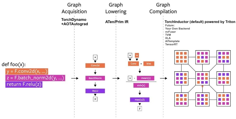
Whenever you wrap your model under torch.compile, the model goes through the following steps before execution (Figure 3):

1. Graph Acquisition: The model is broken down and re-written into subgraphs. Subgraphs that can be compiled/optimized are flattened, whereas other subgraphs which can’t be compiled fall back to the eager model.
2. Graph Lowering: All PyTorch operations are decomposed into their chosen backend-specific kernels.
3. Graph Compilation: All the backend kernels call their corresponding low-level device operations.

Now, let’s start some experimentation.

---

Accelerating DNNs with PyTorch 2.0

---

Project Structure

We first need to review our project directory structure.

Start by accessing the “Downloads” section of this tutorial to retrieve the source code.

From there, take a look at the directory structure:

├── cnn.py
├── vit.py
├── bert.py
├── utils.py

The project directory contains four files. The utils.py file implements basic utility functions to parse command line arguments and run/report a model’s speed. The cnn.py, vit.py, and bert.py files load a specified CNN (convolutional neural network), ViT (vision transformer), or a BERT (bidirectional encoder representations from transformers) model, compile it with torch.compile, and report its speed on a random input. We will discuss these files in detail in subsequent sections.

---

Accelerating Convolutional Neural Networks

Using torch.compile is easy and is expected to provide 30%-200% speedups on most models you run daily. However, first, we will look into some utility functions in utils.py to parse command line arguments and run a model on a given input.

---

Parsing Command Line Arguments and Running a Model

import torch
import time
import numpy as np
import argparse

# command line arguments
def parse_args():
    parser = argparse.ArgumentParser()
    parser.add_argument('--model', type=str, help='model type', default='resnet50')
    parser.add_argument('--batch_size', type=int, help='Batch size', default=128)
    parser.add_argument('--steps', type=int, help='Steps', default=10)
    parser.add_argument('--mode', type=str, help='Mode', default='default')
    parser.add_argument('--backend', type=str, help='Backend', default='inductor')

    args = parser.parse_args()
    return args

# running a model
def run_model(model, inputs, steps=20):
    # load model on GPU
    model = model.cuda() 
    # define an optimizer
    optimizer = torch.optim.Adam(model.parameters()) 
    times = []
    for step in range(steps):
        begin = time.time()
        # zero gradients
        optimizer.zero_grad() 
        # forward pass
        output = model(inputs.cuda()) 
        # back propagate 
        if not isinstance(output, torch.Tensor):
            output = output.logits
        output.sum().backward() 
        # optimize weights
        optimizer.step() 
        end = time.time()
        # calcuate step time
        times.append(float(end - begin)) 
        print(f"Time for {step}-th forward pass is {end - begin}")
    
    # calcuate median step time
    median = np.median(times) 
    print("Median step time is {:.3f} seconds".format(median))

On Lines 1-4, we import the torch, time, argparse, and numpy libraries. Then, on Lines 7-16, we define the parse_args() function that parses the following command line arguments:

• --model: specifies the model to load (default set to resnet50)
• --batch_size: specifies the batch size of the inputs (default set to 128)
• --steps: specifies the number of steps to run the model (default is set to 10)
• --mode: specifies whether to use default, reduce-overhead, or original mode for compilation. We won’t experiment with the max-autotune mode as it takes very long to compile and doesn’t always work.
• --backend: specifies the compiler backend (default set to inductor)

Then on Lines 19-44, we define the run_model() function that takes model, inputs, and steps as arguments and runs the model training on inputs for a given number of steps. First, on Line 21, we load the model on the GPU. Then on Line 23, we define optimizer over model parameters.

Finally, on Lines 25-40, we run the model training for given steps wherein we pass the given inputs, backpropagate gradients, and update network weights in each step. We print and store the time taken by each step in a list of times. Finally, on Lines 43 and 44, we calculate and print the median step time taken by our compiled model.

Now let’s start experimenting with convolutional neural networks.

---

Evaluating Convolutional Neural Networks

import torch
from utils import parse_args, run_model

args = parse_args()

# loading pretrained resnet50
model = torch.hub.load('pytorch/vision:v0.10.0', args.model, pretrained=True) 

# compile your model
if args.mode in ['default', 'reduce-overhead']:
        model = torch.compile(model, mode=args.mode, backend=args.backend)   

# random input image
inputs = torch.randn(args.batch_size, 3, 224, 224) 
run_model(model, inputs, args.steps)

We start by loading the torch library and utilities from utils.py (Lines 1 and 2). On Line 4, we read the command line arguments. Then on Line 7, we load the given args.model from TorchHub. If you are unfamiliar with TorchHub, we highly recommend watching our tutorials.

On Lines 10 and 11, we compile the model using torch.compile with specified mode args.mode. Note that if a user specifies any other mode apart from default and reduce-overhead, we return the original model. By default, we use the inductor backend. On Line 14, we define a random input image with a given batch size args.batch_size. Finally, on Line 15, we run and report the time taken by the model using the run_model utility function.

Here is a sample command to run the above code snippet. The following command tests a ResNet-50 model with default mode and batch size 256.

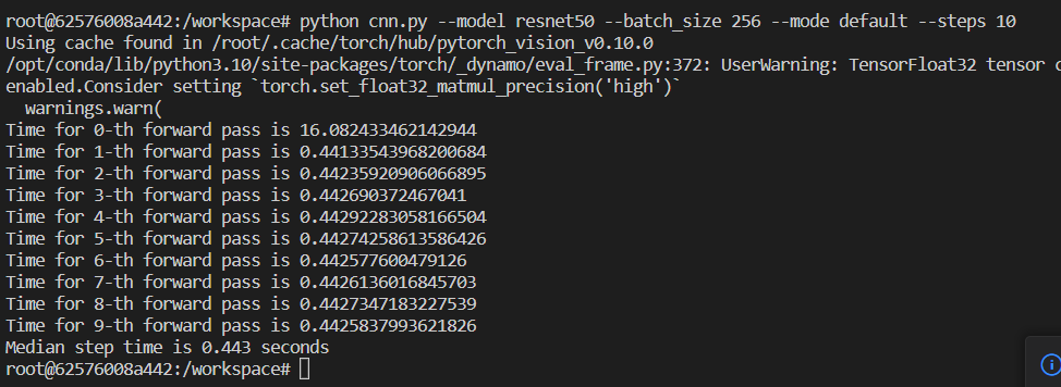
$ python cnn.py --model resnet50 --batch_size 256 --mode default --steps 10

Figure 4 displays how the output should look. Note that your numbers might differ depending on your GPU specs.

When you run the above code snippet, you will notice that the first step takes an abnormally long time while the subsequent steps are faster. This is because the torch.compile is a lazy wrapper and only compiles the model during the first forward pass.

To notice the speedup, you will need to compare the speed of the compiled model with the original model (by using --mode original in the command).

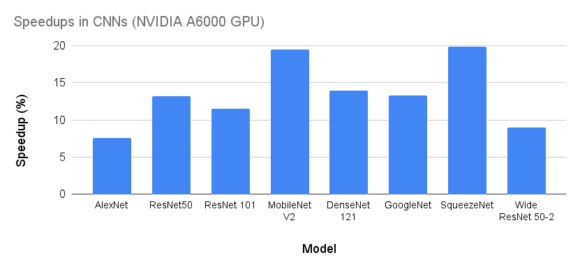
In Figure 5, we compare several convolutional models like ResNets, GoogleNet, AlexNet, SqueezeNet, DenseNet, MobileNet, and Wide ResNet. On average, CNNs give a 10% training speedup on NVIDIA A6000s. Among all the models, MobileNetV2 and SqueezeNet provide close to 20% speedup, while AlexNet and Wide ResNet give <10% speedup. Please note that the speedup might differ depending on your hardware accelerator. You are likely to see more significant speedups with newer GPUs like A100s.

---

Accelerating Vision Transformers

Similarly, using the torch.compile wrapper, one can speed up a vision transformer for image classification tasks. We will use the PyTorch image models (timm) library that can be installed via pip:

$ pip install timm

For this example, we will refer to the vit.py file in our project directory.

---

Evaluating Vision Transformers

import torch
import timm
from utils import parse_args, run_model

args = parse_args()

# loading pretrained ViT model
model = timm.create_model(args.model, pretrained=True) 

# compile your model
if args.mode in ['default', 'reduce-overhead']:
        model = torch.compile(model, mode=args.mode, backend=args.backend)   

# random input image
inputs = torch.randn(args.batch_size, 3, 224, 224) 
run_model(model, inputs, args.steps)

Like our previous example, we start by loading torch, the timm library, and utilities from utils.py (Lines 1-3). Next, on Line 5, we read the command line arguments. Then on Line 8, we load the given args.model from TIMM. The remainder of the code is the same.

Here’s a sample command to run the above code snippet. The following command tests a ViT-B/16 (vision transformer base architecture and patch size 16) model with default mode and batch size 256. You can check out the list of available models using timm.list_models().

$ python vit.py --model vit_base_patch16_224 --batch_size 256 --mode default --steps 10

In Figure 6, we compare several state-of-the-art vision transformers. We notice that, on average, transformers give only 2%-3% speedup compared to >10% speedup for CNNs. This is likely because of the self-attention module, which operates on the global view of the image rather than the local view (e.g., convolutions in CNNs). Hence are difficult to optimize. Models (e.g., MLP-Mixer) give negative speedup, on the other hand.

---

Accelerating BERT

A similar concept works for natural language processing (NLP) models like BERT. We will use the Hugging Face transformers library that can be installed via pip:

$ pip install transformers==4.26.1

For this example, we will refer to the bert.py file in our project directory.

---

Evaluating BERT

import torch
from transformers import AutoConfig, AutoTokenizer, AutoModelForSequenceClassification
from utils import parse_args, run_model

args = parse_args()

# loading pretrained BERT model
config = AutoConfig.from_pretrained(args.model)
tokenizer = AutoTokenizer.from_pretrained(args.model)
model = AutoModelForSequenceClassification.from_config(config)

# compile your model
if args.mode in ['default', 'reduce-overhead']:
        model = torch.compile(model, mode=args.mode, backend=args.backend)   

# random input text
text = ", ".join(["This is a very long text" for i in range(20)])
inputs = tokenizer(text, return_tensors='pt')
inputs = inputs["input_ids"].repeat(args.batch_size, 1)
run_model(model, inputs, args.steps)

On Lines 1-3, we import the torch, transformers, and utils.py libraries. Next, on Line 5, we read the command line arguments. Then, on Lines 8-10, we load the given args.model and its config and tokenizer from the Hugging Face transformers library.

On Lines 13 and 14, we compile the model using torch.compile with specified mode args.mode. Then on Lines 17-19, we define a dummy tokenized input text with a given batch size args.batch_size. Finally, on Line 20, we run and report the time taken by the model using the run_model utility function.

Here’s a sample command to run the above code snippet. The following command tests a BERT model with default mode and batch size 256.

$ python bert.py --model bert-base-uncased --batch_size 256 --mode default --steps 10

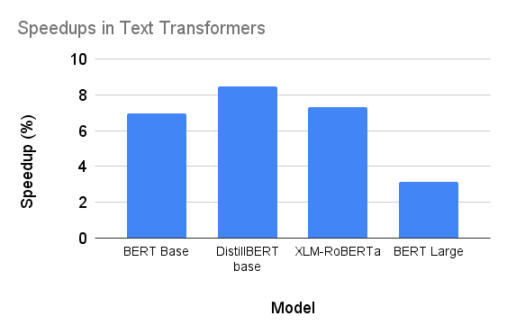
Figure 7 compares some of the state-of-the-art NLP models (e.g., BERT, DistillBERT, and XLM-RoBERTa) from the Hugging Face library. On average, PyTorch 2.0 provides a 5%-6% speedup on these models. On the other hand, DistillBERT achieves a maximum speedup of 8.5%.

---

Miscellaneous

Different Benchmarks: Figure 8 shows the speedup of PyTorch 2.0 on NVIDIA A100 GPUs across 163 open source models from different libraries (e.g., TIMM, TorchBench, and Hugging Face). At Float32 precision, it runs 21% faster on average, and at AMP (automatic mixed precision), it runs 51% faster on average. The figure reports the uneven weighted average speedup of 0.75 * AMP + 0.25 * float32 since we find AMP is more common in practice.

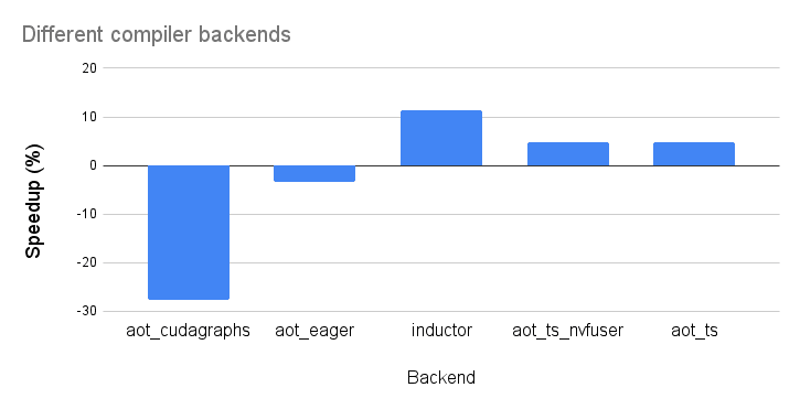
Different Backends: By default, we have used the “inductor” compiler backend in our experiments so far. However, there are plenty of backends supported by PyTorch 2.0. You can find the list of supported backends using torch._dynamo.list_backends(). Figure 9 compares a few different compiler backends with the default TorchInductor backend for the ResNet-50 model. We can see that TorchInductor, by default, gives the maximum speedup.

You can experiment with other backends. Note that these backends are hardware-dependent; some might not work on your hardware.

---

---

Summary

PyTorch has been one of the most popular and widely used frameworks for training and deploying deep learning models. Continuous innovation in PyTorch has resulted in an elegant, high-performance, and eager execution framework. PyTorch 2.0, a next-generation release, brings significant speedup in eager execution by leveraging the best of hardware accelerators through the latest technologies (e.g., TorchDynamo, TorchInductor, PrimTorch, and AOT Autograd).

At the core, PyTorch 2.0 introduces torch.compile, a function that wraps your nn.Module instances, optimizes its graph, and provides a fast model for several backends and architectures. Besides being easy to use, torch.compile is backward compatible. All other operations (e.g., reading and updating attributes, serialization, distributed learning, inference, export, etc.) would work just as in PyTorch 1.x.

On 163 open source models from different libraries (e.g., TIMM, TorchBench, and Hugging Face), torch.compile provided 30%-200% speedups on NVIDIA A100s. Moreover, at Float32 precision, it runs 21% faster on average, and at AMP (automatic mixed precision), it runs 51% faster on average. We also experimented on NVIDIA A6000s and observed that PyTorch 2.0 could provide up to 20% speedup on vision architectures (e.g., SqueezeNet, DenseNet, etc.).

PyTorch has always strived for high performance and eager execution while delivering some of the best abstractions for distributed learning, data loading, and automatic differentiation. With this new release, training deep neural networks in eager modes will become much faster!

---

Citation Information

Mangla, P. “What’s New in PyTorch 2.0? torch.compile,” PyImageSearch, P. Chugh, A. R. Gosthipaty, S. Huot, K. Kidriavsteva, R. Raha, and A. Thanki, eds., 2023, https://pyimg.co/fh15d

@incollection{Mangla_2023_PT2TC,
  author = {Puneet Mangla},
  title = {What's New in PyTorch 2.0? torch.compile},
  booktitle = {PyImageSearch},
  editor = {Puneet Chugh and Aritra Roy Gosthipaty and Susan Huot and Kseniia Kidriavsteva and Ritwik Raha and Abhishek Thanki},
  year = {2023},
  url = {https://pyimg.co/fh15d},
}

---

---

To download the source code to this post (and be notified when future tutorials are published here on PyImageSearch), simply enter your email address in the form below!