Understanding a Real-Time Object Detection Network: You Only Look Once (YOLOv1)

---

---

Understanding a Real-Time Object Detection Network: You Only Look Once (YOLOv1)

Object detection has become increasingly popular and has grown widely, especially in the Deep Learning era. From our previous post, “Introduction to YOLO family,” we know that object detection is divided into three classes of algorithms: traditional computer vision, two-stage detectors, and single-stage detectors.

And today, we are going to discuss one of the first single-stage detectors called Understanding a Real-Time Object Detection Network: You Only Look Once (YOLOv1). YOLOv1, an anchor-less architecture, was a breakthrough in the Object Detection regime that solved object detection as a simple regression problem. It was many times faster than the popular two-stage detectors like Faster-RCNN but at the cost of lower accuracy.

A comprehensive object-annotated image dataset is essential for grasping the YOLOv1 object detection model. It helps in understanding how the model detects and classifies multiple objects in a single pass.

Roboflow has free tools for each stage of the computer vision pipeline that will streamline your workflows and supercharge your productivity.

Sign up or Log in to your Roboflow account to access state of the art dataset libaries and revolutionize your computer vision pipeline.

You can start by choosing your own datasets or using our PyimageSearch’s assorted library of useful datasets.

Bring data in any of 40+ formats to Roboflow, train using any state-of-the-art model architectures, deploy across multiple platforms (API, NVIDIA, browser, iOS, etc), and connect to applications or 3rd party tools.

This lesson is the second part of our seven-part series on YOLO:

1. Introduction to the YOLO Family
2. Understanding a Real-Time Object Detection Network: You Only Look Once (YOLOv1) (this tutorial)
3. A Better, Faster, and Stronger Object Detector (YOLOv2)
4. Mean Average Precision (mAP) Using the COCO Evaluator
5. An Incremental Improvement with Darknet-53 and Multi-Scale Predictions (YOLOv3)
6. Achieving Optimal Speed and Accuracy in Object Detection (YOLOv4)
7. Training the YOLOv5 Object Detector on a Custom Dataset

Today’s post will discuss one of the first single-stage detectors (i.e., YOLOv1) that detects objects at very high speed and yet achieves decent accuracy.

Understanding object detection architecture can be daunting at times.

But don’t worry, we will make it very easy for you, and we will unravel every minute detail that would help you speed up your learning about this topic!

To learn all about the YOLOv1 object detector and see a demo of detecting objects in real-time, just keep reading.

---

Understanding a Real-Time Object Detection Network: You Only Look Once (YOLOv1)

In this second part of the YOLO series, we will first discuss what Single-Stage Object Detectors are. Then, we will give a short introduction to YOLOv1 and discuss its end-to-end detection process.

From there, we’ll compare YOLOv1 with other architectures, understand the network architecture along with the training process, and the combined loss function for detection and classification. Finally, we will review the qualitative and quantitative benchmarks and reflect on YOLOv1 limitations and generalizability of natural and art images.

Finally, we will wrap up this tutorial by installing the darknet framework on the Tesla V100 GPU and running inference on images and a video with the YOLOv1 pretrained model.

---

Configuring Your Development Environment

To follow this guide, you need to have the Darknet Framework compiled and installed on your system. We will use AlexeyAB’s Darknet Repository for this tutorial.

We cover the step-by-step instructions on how to install the darknet framework on Google Colab. However, if you would like to configure your development environment now, consider heading to the Configuring the Darknet Framework and Running Inference with the Pretrained YOLOv1 model section.

---

Having Problems Configuring Your Development Environment?

All that said, are you:

• Short on time?
• Learning on your employer’s administratively locked system?
• Wanting to skip the hassle of fighting with the command line, package managers, and virtual environments?
• Ready to run the code right now on your Windows, macOS, or Linux system?

Then join PyImageSearch University today!

Gain access to Jupyter Notebooks for this tutorial and other PyImageSearch guides that are pre-configured to run on Google Colab’s ecosystem right in your web browser! No installation is required.

And best of all, these Jupyter Notebooks will run on Windows, macOS, and Linux!

---

What Are Single-Stage Object Detectors?

Single-Stage Object Detectors are a class of object detection architectures that are one-stage. They treat object detection as a simple regression problem; for example, the input image is fed to the network, directly outputs the class probabilities and bounding box coordinates.

These models skip the region proposal stage, also known as Region Proposal Network, which is generally part of Two-Stage Object Detectors that are areas of the image that could contain an object.

Figure 2 shows the single-stage and two-stage detector workflow. In single-stage, we apply the detection head directly on the feature map, while, in two-stage, we first apply a region-proposal network on the feature maps.

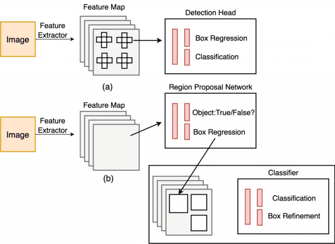
Then, these regions are further passed to the second stage that makes predictions for each region. Faster-RCNN and Mask-RCNN are some of the most popular two-stage object detectors.

While two-stage detectors are considered more accurate than single-stage object detectors, they have a slower inference speed involving multiple stages. On the other hand, single-stage detectors are much faster than two-stage detectors.

---

You Only Look Once (YOLO)

A group of authors led by Joseph Redmon published You Only Look Once: Unified, Real-Time Object Detection at the 2016 CVPR conference.

You only look once or popularly known as YOLO, was a breakthrough in the object detection field. It was the first approach that treated object detection as a regression problem. Using this model, you only look once at an image to predict what objects are present and where they are.

Unlike the two-stage detector approach, YOLO does not have a proposal generator and refine stages; it uses a single neural network that predicts class probabilities and bounding box coordinates from an entire image in one pass. It can be optimized end-to-end since the detection pipeline is essentially one network; think of it as an image classification network.

Since the network is designed to train in an end-to-end fashion similar to image classification, the architecture is extremely fast, and the base YOLO model predicts images at 45 FPS (Frames Per Second) benchmarked on a Titan X GPU. The authors also came up with a much lighter version of YOLO called Fast YOLO, having fewer layers that process images at 155 FPS. Isn’t that amazing?

YOLO achieved 63.4 mAP (mean average precision), more than double the other real-time detectors, making it even more special.

We have an upcoming blog post on mAP using the COCO Evaluator, so do check that out if you are interested to learn how mAP is computed.

Though YOLO makes more localization errors (false negatives), especially small objects compared to other state-of-the-art models like Faster-RCNN, it does well on predicting fewer false positives in the background. However, YOLO still lags behind state-of-the-art detection systems in accuracy like Faster-RCNN. While it can quickly identify objects in images, it struggles to localize some objects, especially small ones.

Another exciting finding from Redmon et al. (2016) was the generalizability of YOLO on artwork and natural images from the internet. Furthermore, it outperformed detection methods like the Deformable Parts Model (DPM) and Region-Based Convolutional Neural Networks (RCNN) by a considerable margin.

---

End-to-End Unified Detection Process

YOLO works on the single-stage detection principle meaning it unifies all the components of the object detection pipeline into a single neural network. It uses the features from the entire image to predict class probabilities and bounding box coordinates.

This approach helps model reason globally about the whole image and the objects in that image. However, in prior two-stage detectors like RCNN, we have a proposal generator that generates rough proposals for the image, which are then passed onto the next stage for classification and regression.

Figure 4 shows that the entire detection process consists of three steps: resizing the input image to , running a single convolutional network on the complete image, and thresholding the resulting detections by the model’s confidence, thereby removing duplicate detections.

This end-to-end unified detection design enables the YOLO architecture to train faster and achieve real-time speed during inference while ensuring high-average precision (close to two-stage detectors).

Traditional methods (e.g., DPM) used the sliding window approach. However, the classifier is run at evenly spaced locations over the entire image, thus making it very slow at training and test time and challenging to optimize, especially the RCNN architectures, since each stage needs to be trained separately.

We learned that YOLO works on the unified end-to-end detection methodology, but how does it accomplish this? Let’s find out!

The YOLO model divides the image into an grid, shown in Figure 5, where . If the center of an object falls into one of the 49 grids, then that cell is responsible for detecting that object.

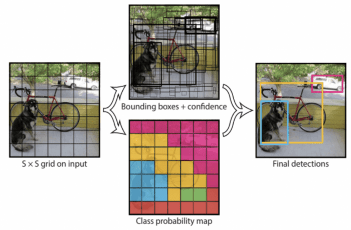
But how many objects can a grid cell be accountable for detecting? Well, each grid cell can detect B bounding boxes and confidence scores for those bounding boxes, .

In total, the model can detect bounding boxes; however, later, we will see that during the training, the model tries to suppress one of the two boxes in each cell that has less Intersection over Union (IOU) with the ground-truth box.

A confidence score is assigned to each box which tells how confident the model is that the bounding box contains an object.

The confidence score can be defined as:

where is 1 if the object exists, and 0 otherwise; when an object is present, the confidence score equals the IOU between the ground truth and the predicted bounding box.

This makes sense because we do not want the confidence score to be 100% (1) when the predicted box is not entirely aligned with the ground-truth box, which allows our network to predict more realistic confidence for each bounding box.

Each bounding box outputs five predictions: .

• The target coordinates represent the center of the bounding box relative to the bounds of the grid cell, meaning the value of would range between [0, 1]. An with value (0.5, 0.5) would mean the object’s center is the center of a particular grid cell.

• The target is the width and height of the bounding box relative to the entire image. This means that the predicted will also be relative to the whole image. The width and height of the bounding box can be greater than 1.

• is the confidence score predicted by the network.

Apart from the bounding box coordinates and confidence score, each grid cell predicts conditional class probabilities , where for PASCAL VOC classes. is conditioned on the grid cell containing an object; hence, it only exists when there is an object.

We learned each grid cell is responsible for predicting two boxes. However, only one with the highest IOU with ground truth is considered; hence, the model predicts one set of class probabilities per grid cell, ignoring the number of boxes .

To develop more intuition, refer to Figure 6; we can observe grids, and each grid cell has output predictions for Box 1 and Box 2 and class probabilities.

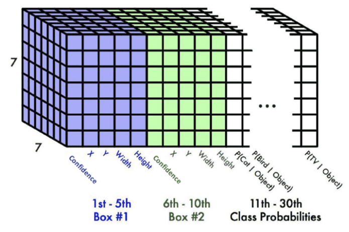
Each bounding box has five values in total ten values for both bounding boxes and 20 class probabilities. Hence, the final prediction is a tensor.

---

Comparing YOLOv1 with Other Architectures

This section compares the YOLO detection architecture to several top detection frameworks like DPM, RCNN, Overfeat, etc.

• DPM: Girshick, Iandola, et al. (2014) use a sliding window approach where each image region was classified depending on the window’s stride. The pipeline was disjoint involving extracting static features, classifying regions, and predicting high-scoring regions.
  
  However, in YOLO, Redmon et al. use a unified approach in which a single CNN model extracts features to perform bounding box prediction and non-maximum suppression. It’s also important to note that YOLO does not depend on static features; they are learned with network training.
  
  Plus, YOLO focuses on the global contextual information rather than just the local regions, as seen in DPM, which helps reduce false positives. Unfortunately, compared to the benchmarks, DPM is way behind the YOLO network both in speed and accuracy.

• RCNN (Girshick, Donahue, et al., 2014): family used region proposals to find objects in images. The selective search was used in RCNN to generate potential bounding boxes. A CNN extracted features from each region, Support Vector Machine (SVM) classified the boxes, and a fully connected linear layer calibrated the bounding boxes. It had so many components, which made it hard to optimize and slow to train.
  
  RCNN took more than 45 seconds which is a lot for an application requiring real-time speed. In addition, RCNN’s selective search approach proposed 2000 bounding boxes compared to YOLO with 98 proposals per image. YOLO combined all these disjoint steps into one single end-to-end joint optimized model.

• Overfeat: Sermanet et al. (2014) used a similar approach as DPM (i.e., sliding window detection but performed it efficiently). It trained a CNN to perform localization, was unable to learn the global context, and required a lot of postprocessing to produce coherent detections. Overall it was also a disjoint architecture.

• Faster-RCNN (Ren et al., 2016): was way better than RCNN. It eliminated selective search for proposing regions but still had two different networks for object detection. It was hard to optimize as it had four loss functions: two for the region proposal network and two for the Fast R-CNN.
  
  It used quite a few fully connected layers, which increased the parameters and reduced the inference time. As a result, Faster-RCNN achieved 5-6 FPS far less than YOLO, although Faster-RCNN surpasses YOLO in mAP.

After comparing YOLO with four different architectures, we can conclude that most of these architectures focused on learning local information and not global. They looked at only the parts of the image and not the image as a whole. The object detection pipeline was not end-to-end; various components could have made these networks hard to optimize and slower at test time.

On the other hand, YOLO did an excellent job of treating object detection as a regression or an image classification problem by designing a single convolutional neural network for performing detection and classification simultaneously.

---

Network Architecture of YOLO

The network architecture of YOLO is straightforward, trust me! It is similar to an image classification network you might have trained in the past. But, to your surprise, this architecture is inspired by the GoogLeNet model used in the image classification task.

It consists of mainly three types of layers: Convolutional, Maxpool, and Fully Connected. The YOLO network has 24 convolutional layers, which do the image feature extraction followed by two fully connected layers for predicting the bounding box coordinates and classification scores.

Redmon et al. modify the original GoogLenet architecture. First, they use the convolutional layers instead of inception modules for reducing feature space, followed by a convolutional layer (see Figure 7).

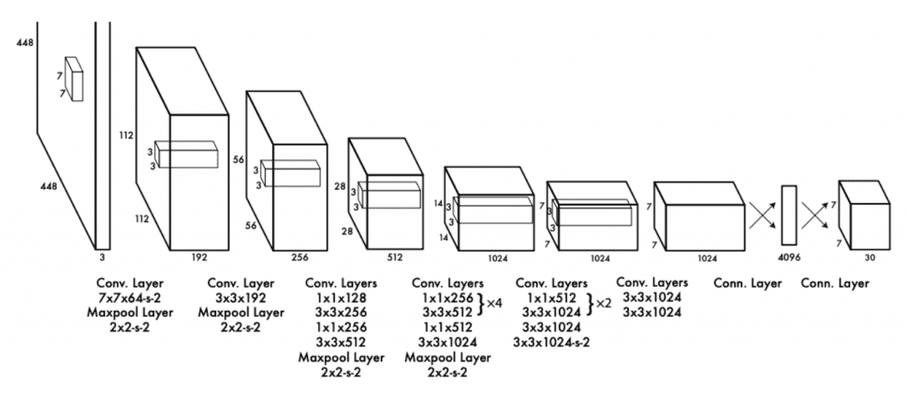
The second variant of YOLO, called Fast-YOLO, has nine convolutional layers instead of 24 and uses a smaller filter size. It was mainly designed to further push the inference speed to an extent one could never imagine. With this setting, the authors were able to achieve 155 FPS!

---

Training Process

As a first step, Redmon et al. trained the network on the ImageNet 1000-class dataset. Then, in the pretraining step, they considered up to the first 20 convolutional layers, followed by average pooling and a fully connected layer.

They trained this model for almost seven days and achieved a top-5 accuracy of 88% on the ImageNet validation set. It was trained with an input resolution of , half the resolution used for object detection. Figure 8 shows the network summary of YOLOv1 that has the detection layer at the end.

The PASCAL VOC 2007 and 2012 datasets were used to train the neural network for the detection task. The network was trained for approximately 135 epochs with a batch size of 64 and a momentum of 0.9. The learning rate varied as the training progressed from to . Standard data augmentation and dropout techniques were used to avoid overfitting.

The authors wrote their framework for training and testing the model known as Darknet written in C language. The pre-trained classification network was stacked with four convolutional and two fully connected layers with random initialization for the detection task.

Since detection is a much more challenging task and requires fine-grained contextual information, the input was upsampled to .

The ground-truth bounding box height and width were normalized to by dividing it with the image height and width. All the layers except the last used LeakyReLU as the activation function with , and the final layer is linear.

---

Loss Function

Let’s now dissect the loss function of YOLO shown in Figure 9. At first glance, the below equation might look a bit lengthy and tricky, but don’t worry; it is straightforward to understand.

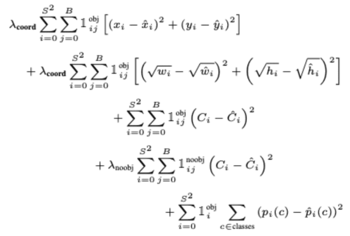
You will notice in this loss equation that we are optimizing the network with the Sum-Squared Error (SSE), and Redmon et al. believe that it is easy to optimize. However, there are a few caveats of using it, which they try to overcome by adding a weight term called .

Let’s understand the above equation part by part:

• The first part of the equation computes the loss between the predicted bounding box midpoints (, ) and the ground-truth bounding box midpoints (, ).
  
  It is calculated for all the 49 grid cells, and only one of the two bounding boxes is considered in the loss. Remember, it only penalizes bounding box coordinate error for the predictor that is “responsible” for the ground-truth box (i.e., has the highest IOU of any predictor in that grid cell).
  
  In short, we will see out of the two bounding boxes which have the highest IOU with the target bounding box, and that will get prioritized for the loss computation.
  
  Finally, we weigh the loss with a constant to ensure that our bounding box predictions are as close as possible to the target. Lastly, an identity function denotes that the th bounding box predictor in cell is responsible for that prediction. Thus, it will be 1 if the target object exists and 0 otherwise.

• The second part is quite similar to the first, so let’s understand the differences. Here, we compute the loss between the predicted bounding box width and height and the target width and height .
  
  But notice we take the square root of width and height (i.e., because sum squared loss equally weighs errors in large and small scale boxes).
  
  A significant deviation in small boxes would be small, whereas a small variation in larger boxes would be significant, which would cause small boxes to matter less. Hence, the authors added a square root to reflect slight deviations in large boxes matter less than in small boxes.

• In the third part of the equation given an object exists , we compute the loss between the predicted confidence score of the bounding box and the target confidence score .
  
  Here, the target confidence score equals the IOU between the predicted bounding box and target. We choose the confidence score of the box that has a higher IOU with the target.

• Next, if no object exists in the grid cell , then and will make the third part of the equation zero. The loss is computed between the box with a higher IOU and the target , which is 0 since we want the confidence for the cell with no object to be 0.
  
  We also weigh this part with since there can be many grid cells with no objects, and we do not want this term to overpower the gradients for the cells containing objects. As highlighted in the paper, this could lead to model instability and be harder to optimize.

• Finally, for every cell, if an object appears in cell , we compute the loss for all 20 classes (conditional class probability). Here, is the predicted conditional class probability, and is the target conditional class probability.

---

Quantitative Benchmarks

Now that we have covered almost all the aspects of the YOLO architecture, let’s look at some quantitative benchmarks that YOLO and its variant Fast YOLO achieved compared to other real-time and non-real-time object detectors.

Table 1 has four attributes: real-time detectors, training data, evaluation metric, and FPS; we use these four attributes for the quantitative comparison. The training data used for training all four models is Pascal VOC. We can see that both the YOLO and Fast YOLO outperforms the real-time object detector variants of DPM by a considerable margin in terms of mean average precision (nearly 2x) and FPS.

The Fast YOLO with nine convolutional layers achieved an mAP of 52.7 and 155 FPS. On the other hand, YOLO obtained 63.4 mAP and 45 FPS. Both of these models would have been a game-changer back in 2016, a definite choice for an object detection application with target deployment as an embedded or a mobile device, especially the Fast YOLO variant.

In Table 2, we compare YOLO with other non-real-time object detectors. Faster-RCNN performs the best in terms of mAP but achieves just 7 FPS, too little for an application that requires real-time processing; add preprocessing and postprocessing, the FPS would reduce even further. While YOLO with VGG-16 as the backbone gets +3% mAP gain compared to the YOLO with GoogLeNet inspired backbone.

---

Generalizability on Art Images

This section discusses Redmon et al.’s generalizability test on YOLO, RCNN, DPM, and two other models. The results were quite interesting, so let’s quickly shed some light on them.

The authors put across an excellent point that the test data doesn’t often come from the same distribution the model has been trained on in a real-world setting, or it could diverge from what the model would have seen before.

Figure 10 shows the qualitative results of YOLOv1 on Art and Natural Images when trained with the Pascal VOC dataset. The model does a pretty good job, although it does think one person is an airplane.

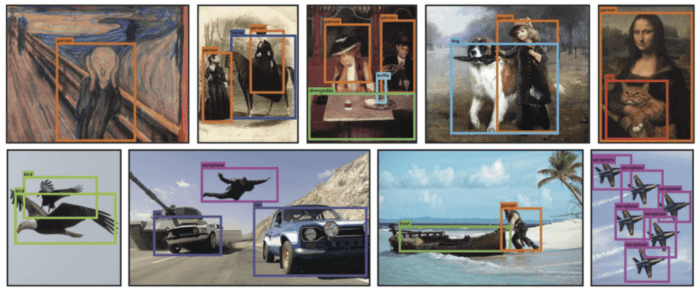
With a similar analogy considering YOLO was trained on the Pascal VOC dataset, they tested the model on two more datasets: Picasso and People-Art Dataset, for testing person detection on artwork.

Table 3 shows a comparison between YOLO and other detection methods. YOLO outperforms the R-CNN and DPM across all three datasets. The VOC 2007 AP is evaluated only on the person class, and all the three models are trained on the VOC 2007 dataset.

For Picasso evaluation, the models were trained on VOC 2012, and for People-Art test data, they were trained on VOC 2010.

Observe that the AP for RCNN on VOC 2007 is high, but the accuracy drops substantially when tested on Picasso and People-Art data. A possible reason for this could be that RCNN uses Selective Search for proposal generation, which is tuned for natural images while this is the artwork. Moreover, the classifier step in RCNN only sees local regions and needs better proposals.

YOLO does well on all three datasets; its AP does not degrade significantly compared to the other two models. The authors state that YOLO learns the size and shape of objects and the relationships between them well. Natural images and artwork might be different on a pixel level, but they are similar semantically, and also the size and shape of objects remain consistent.

---

Limitations of YOLO Architecture

Before discussing the limitations of YOLO, we should all take a moment to appreciate this new single-stage detection technique that made a breakthrough in the object detection domain by offering an architecture that runs so fast and sets new benchmarks!

But nothing is perfect, and there’s always a scope of improvement, and so does YOLOv1.

A few of the limitations are:

1. The model limits the number of objects detected in a given image: a maximum of 49 objects can only be detected.
2. Since each grid cell predicts only two boxes and can only have one class, this limits the number of nearby objects that YOLO can predict, especially the small objects that appear in groups, such as flocks of birds.
3. It also struggles to detect smaller objects. The model uses relatively coarse features for predicting objects since the architecture has multiple downsampling layers from the input image. Hence, a relatively small object would get even smaller at the final layer causing the network harder to localize.
4. Redmon et al. believe that the primary source of error is incorrect localizations since the loss function treats errors the same in small bounding boxes versus large bounding boxes.

This much theory will do. Let’s move on to configuring the darknet framework and running the inference with the pretrained YOLOv1 model.

---

Configuring the Darknet Framework and Running Inference with the Pretrained YOLOv1 Model

We have divided the Darknet framework configuration and ran the inference with YOLOv1 on images and videos into 8 easy to follow steps. So, let’s get started!

Note: Please ensure you have the matching CUDA, CUDNN, and NVIDIA Driver Installed on your machine. For this experiment, we use CUDA-10.2, CUDNN-8.0.3. But if you plan to run this experiment on Google Colab, do not worry, as all these libraries come pre-installed with it.

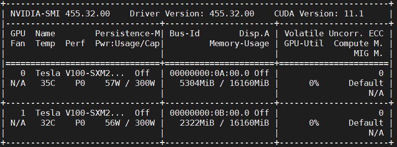
Step #1: We will use the GPU for this experiment to ensure the GPU is up and running.

# Sanity check for GPU as runtime
$ nvidia-smi

Figure 11 shows the GPUs available in machine (i.e., V100), driver, and CUDA versions.

Step #2: We will install a few libraries like OpenCV, FFmpeg, etc., that would be required before compiling and installing darknet.

# Install OpenCV, ffmpeg modules
$ apt install libopencv-dev python-opencv ffmpeg

Step #3: Next, we clone the modified version of the darknet framework from the AlexyAB repository. As learned earlier, Darknet is an open-source neural network written by Joseph Redmon. It is written in C and CUDA, supporting both CPU and GPU computation. The official implementation of the darknet is available at: https://pjreddie.com/darknet/; we will download the YOLOv1 weights provided by the official website.

# Clone AlexeyAB darknet repository
$ git clone https://github.com/AlexeyAB/darknet/
$ cd darknet/

Be sure to change the directory to darknet since, in the next step, we will configure the Makefile and compile it. Do a sanity check using !pwd; we should be in the /content/darknet directory.

Step #4: Using stream editor (sed), we will edit the make files and enable flags: GPU, CUDNN, OPENCV, and LIBSO.

Figure 12 shows a snippet of the Makefile, the contents of which are discussed later:

• We enable the GPU=1 and CUDNN=1 to build darknet with CUDA to perform and accelerate the inference on the GPU. Note CUDA should be in /usr/local/cuda; otherwise, the compilation will result in an error, but don’t worry if you are compiling it on Google Colab.
• If your GPU has Tensor Cores, enable CUDNN_HALF=1 to gain up to 3X inference and 2X training speedup. Since we use a Tesla V100 GPU with tensor cores, we will enable this flag.
• We enable OPENCV=1 to build darknet with OpenCV. This will allow us to detect video files, IP cameras, and other OpenCV off-the-shelf functionalities like reading, writing, and drawing bounding boxes over the frames.
• Finally, we enable LIBSO=1 to build the darknet.so library and binary executable file uselib that uses this library. Allowing this flag to use Python scripts for inference on images and videos will enable us to import darknet inside it.

Now, let’s edit the Makefile and compile it.

# Enable the OpenCV, CUDA, CUDNN, CUDNN_HALF & LIBSO Flags and Compile Darknet
$ sed -i 's/OPENCV=0/OPENCV=1/g' Makefile
$ sed -i 's/GPU=0/GPU=1/g' Makefile
$ sed -i 's/CUDNN=0/CUDNN=1/g' Makefile
$ sed -i 's/CUDNN_HALF=0/CUDNN_HALF=1/g' Makefile
$ sed -i 's/LIBSO=0/LIBSO=1/g' Makefile
$ make

The make command will take around 90 seconds to finish the execution. Now that the compilation is complete, we are all set to download the YOLOv1 weights and run the inference.

Aren’t you excited?

Step #5: We will now download the YOLOv1 weights from the official YOLOv1 documentation.

# Download YOLOv1 Weights
$ wget http://pjreddie.com/media/files/yolov1/yolov1.weights

Step #6: Now, we will run the darknet_images.py script to infer the images.

# Run the darknet image inference script
$ python3 darknet_images.py --in hun put data --weights \ 
yolov1.weights --config_file cfg/yolov1/yolo.cfg \
--data_file cfg/voc.data --dont_show

Let’s put some light on the command line arguments we pass to darknet_images.py:

• --input: Path to the images directory or text file with the path to the images or a single image name. Supports jpg, jpeg, and png image formats. In this case, we pass the path to the image folder called data.
• --weights: YOLOv1 weights path.
• --config_file: Configuration file path for YOLOv1. On an abstract level, this file stores the neural network model architecture and a few other parameters like batch_size, classes, input_size, etc. We recommend you give a quick read of this file by opening it in a text editor.
• --data_file: Here, we pass the Pascal VOC labels file.
• --dont_show: This will disable OpenCV from displaying the inference results, and we use this since we are working with colab.

Below are the object detection inference results by the YOLOv1 model over a set of images.

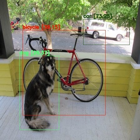
We can see from Figure 13 that the model performed well as it correctly predicted a dog, bicycle, and car.

In Figure 14, the model predicts one false positive by classifying a Horse as a Sheep while correctly predicting the other two objects.

In Figure 15, the model again does a decent job by correctly detecting several horses. However, the localization is not very accurate, and it does miss a couple of horses. In our next post, you will see YOLOv2 does a slightly better job at predicting the below image.

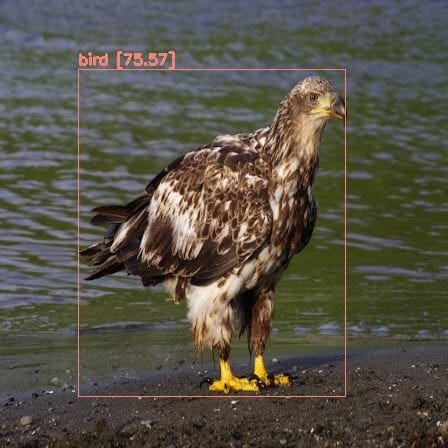
Figure 16 is an image of an Eagle, which is well localized by the model and classified as a Bird. Unfortunately, the Pascal VOC dataset does not have an Eagle class, but the model does a great job predicting it as a bird.

Step #7: Now, we will run the pretrained YOLOv1 model on a video from the movie Skyfall; it is the same video that Redmon et al. had used in one of their experiments with YOLOv1.

Before running the darknet_video.py demo script, we will first download the video from YouTube using the pytube library and crop the video with the moviepy library. So let’s quickly install these modules and download the video.

# Install pytube and moviepy for downloading and cropping the video
$ pip install git+https://github.com/rishabh3354/pytube@master
$ pip install moviepy

# Import the necessary packages
$ from pytube import YouTube
$ from moviepy.video.io.ffmpeg_tools import ffmpeg_extract_subclip

# Download the video in 720p and Extract a subclip
$ YouTube('https://www.youtube.com/watch?v=tHRLX8jRjq8'). \ streams.filter(res="720p").first().download()
$ ffmpeg_extract_subclip("/content/darknet/Skyfall.mp4", \ 
0, 30, targetname="/content/darknet/Skyfall-Sample.mp4")

Step #8: Finally, we will run the darknet_video.py script to generate predictions for the Skyfall video. We print the FPS information over each frame of the output video.

Change the video codec in the set_saved_video function from MJPG to mp4v on Line 57 of the darknet_video.py script in the darknet folder if using an mp4 video file; otherwise, you will get a decoding error while playing the inference video.

# Change the VideoWriter Codec
fourcc = cv2.VideoWriter_fourcc(*"mp4v")

Now that all the necessary installations and modifications are complete, we will run the darknet_video.py script:

# Run the darknet video inference script
$ python darknet_video.py --input \ 
/content/darknet/Skyfall-Sample.mp4 \ 
--weights yolov1.weights --config_file \ 
cfg/yolov1/yolo.cfg --data_file ./cfg/voc.data \
--dont_show --out_filename pred-skyfall.mp4

Let’s look at the command line arguments we pass to darknet_video.py:

• --input: path to the video file or 0 if using a webcam
• --weights: YOLO weights path
• --config_file: configuration file path
• --data_file: passes the Pascal VOC labels file
• --dont_show: disables OpenCV from displaying the inference results
• --out_filename: inference results of the output video name if the empty output video is not saved.

Voila! Below are the inference results on the Skyfall Action Scene Video, and the predictions seem to be good. The YOLOv1 network achieves an average of 140 FPS on the Tesla V100 with mixed precision.

---

Summary

This was an essential and detailed topic, and you have learned a lot, so let’s quickly summarize:

1. We started the tutorial by highlighting the importance of Object Detection in Computer Vision, its various industrial applications and discussed the difference between Single-Stage and Two-Stage Detectors.
2. We then introduced you to the first single-stage detector called YOLOv1. We discussed certain key aspects of this architecture and its performance in terms of speed and accuracy.
3. We discussed in detail the End-to-End Unified Detection process of YOLOv1.
4. We then compared YOLOv1 with other object detection architectures like DPM, RCNN and learned that YOLOv1 does better than its predecessors.
5. You then learned the Network Architecture and the Loss Function of YOLOv1 in detail.
6. We discussed the Quantitative Benchmarks and even the Generalizability of YOLOv1 on Art Images, along with few limitations.
7. Finally, we installed and compiled the Darknet Framework to run Inference with the YOLOv1 model on images and video, achieving good detection results with 140 FPS processing speed.

With YOLOv1, you have struck a significant goal. Keep that momentum going as we bring you more exciting posts on YOLO in the future. Congratulations!

---

Citation Information

Sharma, A. “Understanding a Real-Time Object Detection Network: You Only Look Once (YOLOv1),” PyImageSearch, D. Chakraborty, P. Chugh, A. R. Gosthipaty, S. Huot, K. Kidriavsteva, R. Raha, and A. Thanki, eds., 2022, https://pyimg.co/3cpmz

@incollection{Sharma_2022_YOLOv1,
  author = {Aditya Sharma},
  title = {Understanding a Real-Time Object Detection Network: You Only Look Once {(YOLOv1)}},
  booktitle = {PyImageSearch},
  editor = {Devjyoti Chakraborty and Puneet Chugh and Aritra Roy Gosthipaty and Susan Huot and Kseniia Kidriavsteva and Ritwik Raha and Abhishek Thanki},
  year = {2022},
  note = {https://pyimg.co/3cpmz},
}

---