U-Net Image Segmentation in Keras

In this tutorial, you will learn how to create U-Net, an image segmentation model in TensorFlow 2 / Keras. We will first present a brief introduction on image segmentation, U-Net architecture, and then walk through the code implementation with a Colab notebook.

To learn how to implement a U-Net with TensorFlow 2 / Keras, just keep reading.

U-Net Image Segmentation in Keras

Image segmentation is a computer vision task that segments an image into multiple areas by assigning a label to every pixel of the image. It provides much more information about an image than object detection, which draws a bounding box around the detected object, or image classification, which assigns a label to the object.

Segmentation is useful and can be used in real-world applications such as medical imaging, clothes segmentation, flooding maps, self-driving cars, etc.

There are two types of image segmentation:

• Semantic segmentation: classify each pixel with a label.
• Instance segmentation: classify each pixel and differentiate each object instance.

U-Net is a semantic segmentation technique originally proposed for medical imaging segmentation. It’s one of the earlier deep learning segmentation models, and the U-Net architecture is also used in many GAN variants such as the Pix2Pix generator.

U-Net Architecture

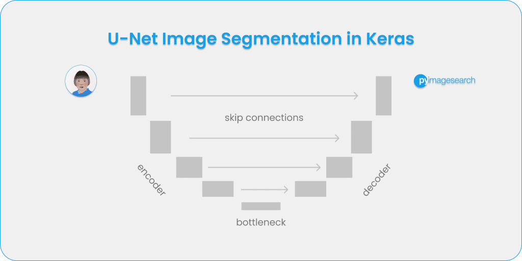
U-Net was introduced in the paper, U-Net: Convolutional Networks for Biomedical Image Segmentation. The model architecture is fairly simple: an encoder (for downsampling) and a decoder (for upsampling) with skip connections. As Figure 1 shows, it shapes like the letter U hence the name U-Net.

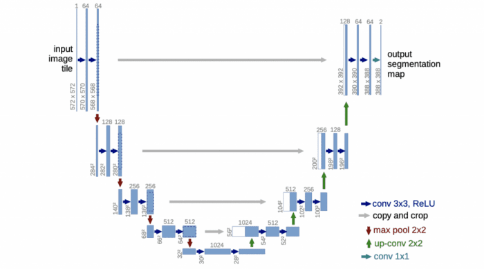
The gray arrows indicate the skip connections that concatenate the encoder feature map with the decoder, which helps the backward flow of gradients for improved training.

Now that we have a basic understanding of semantic segmentation and the U-Net architecture, let’s implement a U-Net with TensorFlow 2 / Keras. Please follow the tutorial below with this Colab notebook.

Setup

We will be using Colab for model training, so make sure you set “Hardware accelerator” to “GPU under Runtime / change runtime type.” Then import the libraries and packages this project depends on:

import tensorflow as tf
from tensorflow import keras
from tensorflow.keras import layers
import tensorflow_datasets as tfds
import matplotlib.pyplot as plt
import numpy as np

Dataset

We will use the Oxford-IIIT pet dataset, available as part of the TensorFlow Datasets (TFDS). It can be easily loaded with TFDS, and then with a bit of data preprocessing, ready for training segmentation models.

With just one line of code, we can use tfds to load the dataset by specifying the name of the dataset, and get the dataset info by setting with_info=True:

dataset, info = tfds.load('oxford_iiit_pet:3.*.*', with_info=True)

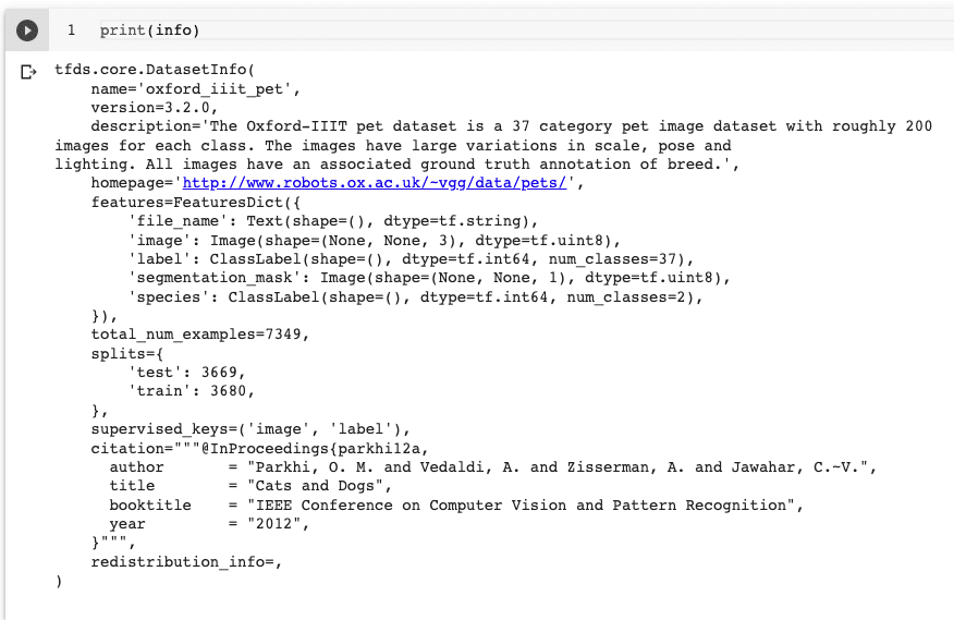
Print the dataset info with print(info), and we will see all kinds of detailed information about the Oxford pet dataset. For example, in Figure 2, we can see there are a total of 7349 images with a built-in test/train split.

Let’s first make a few changes to the downloaded data before we start training U-Net with it.

First, we need to resize the images and masks to 128x128:

def resize(input_image, input_mask):
   input_image = tf.image.resize(input_image, (128, 128), method="nearest")
   input_mask = tf.image.resize(input_mask, (128, 128), method="nearest")

   return input_image, input_mask

We then create a function to augment the dataset by flipping them horizontally:

def augment(input_image, input_mask):
   if tf.random.uniform(()) > 0.5:
       # Random flipping of the image and mask
       input_image = tf.image.flip_left_right(input_image)
       input_mask = tf.image.flip_left_right(input_mask)

   return input_image, input_mask

We create a function to normalize the dataset by scaling the images to the range of [-1, 1] and decreasing the image mask by 1:

def normalize(input_image, input_mask):
   input_image = tf.cast(input_image, tf.float32) / 255.0
   input_mask -= 1
   return input_image, input_mask

We create two functions to preprocess the training and test datasets with a slight difference between the two – we only perform image augmentation on the training dataset.

def load_image_train(datapoint):
   input_image = datapoint["image"]
   input_mask = datapoint["segmentation_mask"]
   input_image, input_mask = resize(input_image, input_mask)
   input_image, input_mask = augment(input_image, input_mask)
   input_image, input_mask = normalize(input_image, input_mask)

   return input_image, input_mask

def load_image_test(datapoint):
   input_image = datapoint["image"]
   input_mask = datapoint["segmentation_mask"]
   input_image, input_mask = resize(input_image, input_mask)
   input_image, input_mask = normalize(input_image, input_mask)

   return input_image, input_mask

Now we are ready to build an input pipeline with tf.data by using the map() function:

train_dataset = dataset["train"].map(load_image_train, num_parallel_calls=tf.data.AUTOTUNE)
test_dataset = dataset["test"].map(load_image_test, num_parallel_calls=tf.data.AUTOTUNE)

If we execute print(train_dataset), we will notice that the image is in the shape of 128x128x3 of tf.float32 while the image mask is in the shape of 128x128x1 with the data type of tf.uint8.

We define a batch size of 64 and a buffer size of 1000 for creating batches of training and test datasets. With the original TFDS dataset, there are 3680 training samples and 3669 test samples, which are further split into validation/test sets. We will use the train_batches and the validation_batches for training the U-Net model. After the training finishes, we will then use the test_batches to test the model predictions.

BATCH_SIZE = 64
BUFFER_SIZE = 1000
train_batches = train_dataset.cache().shuffle(BUFFER_SIZE).batch(BATCH_SIZE).repeat()
train_batches = train_batches.prefetch(buffer_size=tf.data.experimental.AUTOTUNE)
validation_batches = test_dataset.take(3000).batch(BATCH_SIZE)
test_batches = test_dataset.skip(3000).take(669).batch(BATCH_SIZE)

Now the datasets are ready for training. Let’s visualize a random sample image and its mask from the training dataset, to get an idea of how the data looks.​​

def display(display_list):
 plt.figure(figsize=(15, 15))

 title = ["Input Image", "True Mask", "Predicted Mask"]

 for i in range(len(display_list)):
   plt.subplot(1, len(display_list), i+1)
   plt.title(title[i])
   plt.imshow(tf.keras.utils.array_to_img(display_list[i]))
   plt.axis("off")
 plt.show()

sample_batch = next(iter(train_batches))
random_index = np.random.choice(sample_batch[0].shape[0])
sample_image, sample_mask = sample_batch[0][random_index], sample_batch[1][random_index]
display([sample_image, sample_mask])

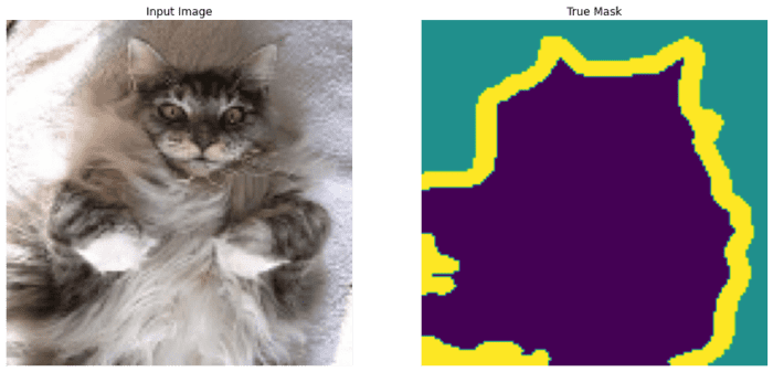
The sample input image of a cat is in the shape of 128x128x3. The true mask has three segments: the green background; the purple foreground object, in this case, a cat; and the yellow outline. Figure 3 shows both the original input image and the true mask image.

Model Architecture

Now that we have the data ready for training, let’s define the U-Net model architecture. As mentioned earlier, the U-Net is shaped like a letter U with an encoder, decoder, and the skip connections between them. So we will create a few building blocks to make the U-Net model.

Building blocks

First, we create a function double_conv_block with layers Conv2D-ReLU-Conv2D-ReLU, which we will use in both the encoder (or the contracting path) and the bottleneck of the U-Net.

def double_conv_block(x, n_filters):

   # Conv2D then ReLU activation
   x = layers.Conv2D(n_filters, 3, padding = "same", activation = "relu", kernel_initializer = "he_normal")(x)
   # Conv2D then ReLU activation
   x = layers.Conv2D(n_filters, 3, padding = "same", activation = "relu", kernel_initializer = "he_normal")(x)

   return x

Then we define a downsample_block function for downsampling or feature extraction to be used in the encoder.

def downsample_block(x, n_filters):
   f = double_conv_block(x, n_filters)
   p = layers.MaxPool2D(2)(f)
   p = layers.Dropout(0.3)(p)

   return f, p

Finally, we define an upsampling function upsample_block for the decoder (or expanding path) of the U-Net.

def upsample_block(x, conv_features, n_filters):
   # upsample
   x = layers.Conv2DTranspose(n_filters, 3, 2, padding="same")(x)
   # concatenate
   x = layers.concatenate([x, conv_features])
   # dropout
   x = layers.Dropout(0.3)(x)
   # Conv2D twice with ReLU activation
   x = double_conv_block(x, n_filters)

   return x

U-Net Model

There are three options for making a Keras model, as well explained in Adrian’s blog and the Keras documentation:

1. Sequential API: easiest and beginner-friendly, stacking the layers sequentially.
2. Functional API: more flexible and allows non-linear topology, shared layers, and multiple inputs or multi-outputs.
3. Model subclassing: most flexible and best for complex models that need custom training loops.

U-Net has a fairly simple architecture; however, to create the skip connections between the encoder and decoder, we will need to concatenate some layers. So the Keras Functional API is most appropriate for this purpose.

First, we create a build_unet_model function, specify the inputs, encoder layers, bottleneck, decoder layers, and finally the output layer with Conv2D with activation of softmax. Note the input image shape is 128x128x3. The output has three channels corresponding to the three classes that the model will classify each pixel for: background, foreground object, and object outline.

 # inputs
   inputs = layers.Input(shape=(128,128,3))

   # encoder: contracting path - downsample
   # 1 - downsample
   f1, p1 = downsample_block(inputs, 64)
   # 2 - downsample
   f2, p2 = downsample_block(p1, 128)
   # 3 - downsample
   f3, p3 = downsample_block(p2, 256)
   # 4 - downsample
   f4, p4 = downsample_block(p3, 512)

   # 5 - bottleneck
   bottleneck = double_conv_block(p4, 1024)

   # decoder: expanding path - upsample
   # 6 - upsample
   u6 = upsample_block(bottleneck, f4, 512)
   # 7 - upsample
   u7 = upsample_block(u6, f3, 256)
   # 8 - upsample
   u8 = upsample_block(u7, f2, 128)
   # 9 - upsample
   u9 = upsample_block(u8, f1, 64)

   # outputs
   outputs = layers.Conv2D(3, 1, padding="same", activation = "softmax")(u9)

   # unet model with Keras Functional API
   unet_model = tf.keras.Model(inputs, outputs, name="U-Net")

   return unet_model

We call the build_unet_model function to create the model unet_model:

unet_model = build_unet_model()

And we can visualize the model architecture with model.summary() to see each detail of the model. And we can use a Keras utils function called plot_model to generate a more visual diagram, including the skip connections. The generated image generated in Colab is rotated 90 degrees so that you can see U-shaped architecture in Figure 4 (see the details better in the Colab notebook):

Compile and Train U-Net

To compile unet_model, we specify the optimizer, the loss function, and the accuracy metrics to track during training:

unet_model.compile(optimizer=tf.keras.optimizers.Adam(),
                  loss="sparse_categorical_crossentropy",
                  metrics="accuracy")

We train the unet_model by calling model.fit() and training it for 20 epochs.

NUM_EPOCHS = 20

TRAIN_LENGTH = info.splits["train"].num_examples
STEPS_PER_EPOCH = TRAIN_LENGTH // BATCH_SIZE

VAL_SUBSPLITS = 5
TEST_LENTH = info.splits["test"].num_examples
VALIDATION_STEPS = TEST_LENTH // BATCH_SIZE // VAL_SUBSPLITS

model_history = unet_model.fit(train_batches,
                              epochs=NUM_EPOCHS,
                              steps_per_epoch=STEPS_PER_EPOCH,
                              validation_steps=VALIDATION_STEPS,
                              validation_data=test_batches)

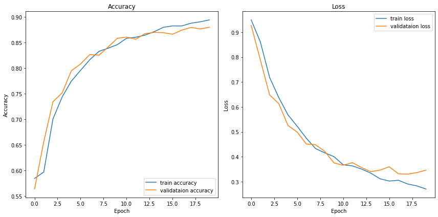
After training for 20 epochs, we get a training accuracy and a validation accuracy of ~0.88. The learning curve during training indicates that the model is doing well on both the training dataset and validation set, which indicates the model is generalizing well without much overfitting (Figure 5).

Prediction

Now that we have completed training the unet_model, let’s use it to make predictions on a few sample images of the test dataset.

def create_mask(pred_mask):
 pred_mask = tf.argmax(pred_mask, axis=-1)
 pred_mask = pred_mask[..., tf.newaxis]
 return pred_mask[0]

def show_predictions(dataset=None, num=1):
 if dataset:
   for image, mask in dataset.take(num):
     pred_mask = unet_model.predict(image)
     display([image[0], mask[0], create_mask(pred_mask)])
 else:
   display([sample_image, sample_mask,
            create_mask(model.predict(sample_image[tf.newaxis, ...]))])

count = 0
for i in test_batches:
   count +=1
print("number of batches:", count)

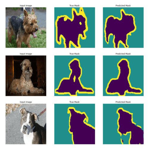
See Figure 6 for the input images, the true masks, and the masks predicted by the U-Net model we trained.

Summary

In this post, you have learned how to load the Oxford-IIIT pet data with the TensorFlow dataset and how to train an image segmentation U-Net model from scratch. We created the U-Net with Keras Functional API and visualized the U-shaped architecture with skip connections. This post has been inspired by the official TensorFlow.org image segmentation tutorial and the U-Net tutorial on Keras.io, which uses keras.utils.Sequence for loading the data and has an Xception-style U-Net architecture. U-Net is a great start for learning semantic segmentation on images. To learn more about this topic, read segmentation papers on modern models such as DeepLab V3, HRNet, U2-Net, etc., among many other papers.

Citation Information

Maynard-Reid, M. “U-Net Image Segmentation in Keras,” PyImageSearch, 2022, https://pyimg.co/6m5br

@article{Maynard-Reid_2022_U-Net,
  author = {Margaret Maynard-Reid},
  title = {{U-Net} Image Segmentation in Keras},
  journal = {PyImageSearch},
  year = {2022},
  note = {https://pyimg.co/6m5br},
}

To download the source code to this post (and be notified when future tutorials are published here on PyImageSearch), simply enter your email address in the form below!