Table of Contents
A few days back, while going through my photo gallery, I came across three pictures shown in Figure 1.

We can see that the pictures are of a staircase but from different viewpoints. I took three pictures because I wasn’t sure I could capture this beautiful scene with just one photo. I was worried I’d miss the right perspective.

This got me thinking, “what if there was a way to capture the entire 3D scene just from these pictures?”
That way, you (my audience) will be able to view exactly what I saw that day.
In NeRF: Representing Scenes as Neural Radiance Fields for View Synthesis, Mildenhall et al. (2020) proposed a method that turned out to be just what I needed.
Let’s look at what we have achieved by reproducing the paper’s method, as shown in Figure 2. For example, giving the algorithm some pictures of a plate of hotdogs from different viewpoints (top) could generate the entire 3D scenery (bottom) precisely.
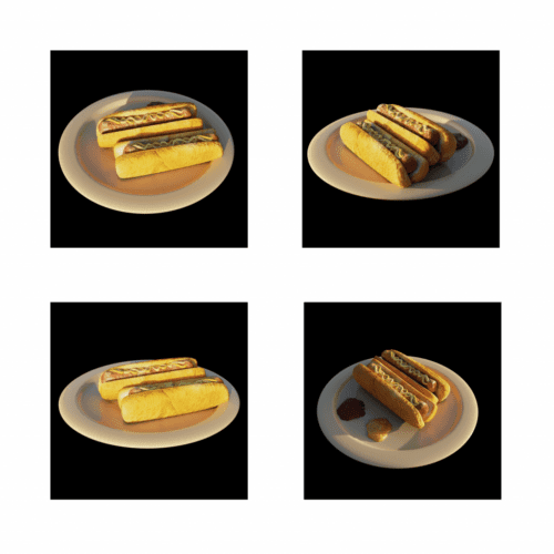
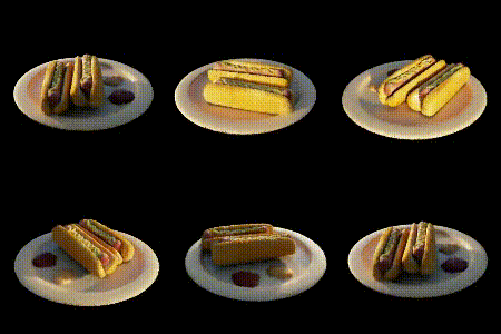
Neural Radiance Fields (NeRF) bring together Deep Learning and Computer Graphics. While we at PyImageSearch have written a lot about Deep Learning, this will be the first time we talk about Computer Graphics. This series will be structured in a way that will best suit an absolute beginner. We expect no prior knowledge of Computer Graphics.
Note: A simpler implementation of NeRF won us the TensorFlow Community Spotlight Award.
To learn about Computer Graphics and image rendering, just keep reading.
Computer Graphics and Deep Learning with NeRF using TensorFlow and Keras: Part 1
Computer Graphics has been one of the wonders of modern technology. The applications of rendering realistic 3D scenes range from movies, space navigation, to medical science.
This lesson is part 1 of a 3-part series on Computer Graphics and Deep Learning with NeRF using TensorFlow and Keras:
- Computer Graphics and Deep Learning with NeRF using TensorFlow and Keras: Part 1 (this tutorial)
- Computer Graphics and Deep Learning with NeRF using TensorFlow and Keras: Part 2 (next week’s tutorial)
- Computer Graphics and Deep Learning with NeRF using TensorFlow and Keras: Part 3
In this tutorial, we will cover the workings of a camera in the world of computer graphics. We will also introduce you to the dataset where we will work.
We have divided this tutorial into the following subsections:
- World Coordinate Frame: representing the physical 3D world
- Camera Coordinate Frame: representing the virtual 3D camera world
- Coordinate Transformation: mapping from one coordinate frame to another
- Projection Transformation: forming an image on a 2D plane (the camera sensor)
- Dataset: understanding the dataset for NeRF
Imagine this. You are out with your camera and spot a beautiful flower. You think about the way you want to capture it. Now it is time to orient the camera, calibrate the settings, and click the picture.
This entire process of transforming the world scene into an image is encapsulated in a mathematical model commonly called the forward imaging model. We can visualize the model in Figure 3.

The forward imaging model starts from a point in the world coordinate frame. We then transform this to the camera coordinate frame using coordinate transformation. After that, we use projection transformation to transform the camera coordinates onto the image plane.
World Coordinate Frame
All shapes and objects that we see in the real world exist in a 3D frame of reference. We call this frame of reference the world coordinate frame. Using this frame, we can locate any point or object in the 3D space quite easily.
Let’s take the point in the 3D space as shown in Figure 4.
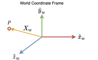
Here, ,
, and
represent the three axes in the world coordinate frame. The location of the point
is expressed through the vector
.
Camera Coordinate Frame
Like the world coordinate frame, we have another frame of reference called the camera coordinate frame, as shown in Figure 5.

This frame sits at the center of a camera. Unlike the world coordinate frame, this is not a static frame of reference. We can move this frame as we are moving the camera around to take a picture.
The same point from Figure 4 can now be located with both frames of reference, as shown in Figure 6.

While in the world coordinate frame, the point is located by the vector, in the camera coordinate frame, it is located by the
vector as shown in Figure 6.
Note: The location of point does not change. Only the way of looking at the point changes with change in the frame of reference.
Coordinate Transformation
We have established two coordinate frames: the world and the camera. Now let us define a mapping between the two.
Let’s take the point from Figure 6. Our goal is to build a bridge between the camera coordinates
and world coordinates
.
From Figure 5, we can say that
where
represents the orientation of the camera coordinate frame with respect to the world coordinate frame. The orientation is represented by a matrix.
→ Direction of
in the world coordinate system.
→ Direction of
in the world coordinate system.
→ Direction of
in the world coordinate system.
represents the position of the camera coordinate frame with respect to the world coordinate frame. The position is represented by a vector.
We can expand the above equation as follows
where represents the translation matrix
. The mapping between the two coordinate systems has been devised but is not yet complete. In the above equation, we have a matrix multiplication along with a matrix addition. It is always preferable to compress things to a single matrix multiplication if we can. To do so we will use a concept called homogeneous coordinates.
The homogeneous coordinate system allows us to represent an dimensional point
in an
dimensional space
with a fictitious variable
such that
Using the homogeneous coordinate system we can transform (3D) to
(4D).
With the homogeneous coordinates at hand, we can compress the equation … to just matrix multiplication.
where is the matrix that holds the orientation and position of the camera coordinate frame. We can call this matrix the Camera Extrinsic since it represents values like rotation and translation, both of which are external properties of the camera.
Projective Transformation
We started with a point and its (homogeneous) world coordinates
. With the help of the camera extrinsic matrix
,
was transformed into its (homogeneous) camera coordinates
.
Now we come to the final stage of actually materializing an image from the 3D camera coordinates as shown in Figure 7.
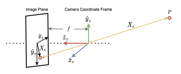
To understand projective transformation, the only thing we need is similar triangles. Let’s do a primer on similar triangles.
We have visualized similar triangles in Figures 8 and 9. With similar triangles
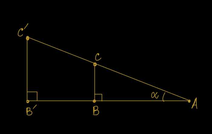
 and
and  are similar triangles.
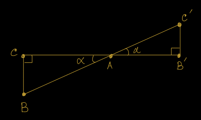
 and
and  are similar triangles.
Yes, you guessed it correctly, and
are similar triangles in Figure 10.
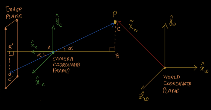
From the properties of similar triangles, we can derive that
Therefore it follows:
Now it is important to remember that the actual image plane is not a virtual plane but rather an array of image sensors. The 3D scene falls on this sensor which leads to the formation of the image. Thus and
in the image plane can be substituted with pixel values
.
A pixel in an image plane starts from the upper left-hand corner (0, 0), so it is also required to shift the pixels with respect to the center of the image plane.
Here, and
are the center points of the image plane.
Now we have a point from the 3D camera space represented in terms of in the image plane. Again to make matrices agree, we have to express the pixel values using homogeneous representation.
Homogeneous representation of , where
and
This can be further expressed as:
Finally, we have:
which can be expressed simply as
where is the set of vectors containing the location of the point in camera coordinate space and
is the set of values containing the location of the point on the image plane. Respectively,
represents the set of values needed to map a point from the 3D camera space to the 2D space.
We can call the camera intrinsic since it represents values like focal length and center of the image plane along
and
axes, both of which are internal properties of the camera.
Dataset
Enough theory! Show me some code.
In this section, we will talk about the data with which we are going to work. The authors have open-sourced their dataset, and you can find it here. The link to the dataset was published in the official repository of NeRF. The dataset is structured as shown in Figure 11.

There are two folders, nerf_synthetic and nerf_llff_data. Moving ahead, we will be using the synthetic dataset for this series.
Let’s see what is in the nerf_synthetic folder. The data in the nerf_synthetic folder is shown in Figure 12.

There are a lot of synthetic objects here. Let’s download one of them and see what is inside. We have chosen the “ship” dataset, but feel free to download any one of them.
After unzipping the dataset, you will find three folders containing images:
trainvaltest
and three files containing the orientation and position of the camera.
transforms_train.jsontransforms_val.jsontransforms_test.json
To better understand the json files, we can open a blank Colab notebook and upload the transforms_train.json. We can now perform exploratory data analysis on it.
# import the necessary packages
import json
import numpy as np

# define the json training file
jsonTrainFile = "transforms_train.json"

# open the file and read the contents of the file
with open(jsonTrainFile, "r") as fp:
    jsonTrainData = json.load(fp)

# print the content of the json file
print(f"[INFO] Focal length train: {jsonTrainData['camera_angle_x']}")
print(f"[INFO] Number of frames train: {len(jsonTrainData['frames'])}")

# OUTPUT
# [INFO] Focal length train: 0.6911112070083618
# [INFO] Number of frames train: 100
We begin with importing the necessary packages json and numpy on Lines 2 and 3.
Then we the load json and read its values on Lines 6-10.
The json file has two parent keys called camera_angle_x and frames. We see that camera_angle_x corresponds to the camera’s field of view, and frames are a collection of metadata for each image (frame).
On Lines 13 and 14, we print the values of the json keys. Lines 17 and 18 show the output.
Let’s investigate frames a little further.
# grab the first frame
firstFrame = jsonTrainData["frames"][0]

# grab the transform matrix and file name
tMat = np.array(firstFrame["transform_matrix"])
fName = firstFrame["file_path"]

# print the data
print(tMat)
print(fName)

# OUTPUT
# array([[-0.92501402,  0.27488998, -0.26226836, -1.05723763],
#       [-0.37993318, -0.66926789,  0.63853836,  2.5740304 ],
#       [ 0.        ,  0.6903013 ,  0.72352195,  2.91661024],
#       [ 0.        ,  0.        ,  0.        ,  1.        ]])
# ./train/r_0
We grab the first frame on Line 20. Each frame is a dictionary containing two keys, transform_matrix and file_path, as shown on Lines 23 and 24. The file_path is the path to the image (frame) under consideration, and the transform_matrix is the camera-to-world matrix for that image.
On Lines 27 and 28, we print the transform_matrix and file_path. Lines 31-35 show the output.
What's next? We recommend PyImageSearch University.
86+ total classes • 115+ hours hours of on-demand code walkthrough videos • Last updated: March 2026
★★★★★ 4.84 (128 Ratings) • 16,000+ Students Enrolled
I strongly believe that if you had the right teacher you could master computer vision and deep learning.
Do you think learning computer vision and deep learning has to be time-consuming, overwhelming, and complicated? Or has to involve complex mathematics and equations? Or requires a degree in computer science?
That’s not the case.
All you need to master computer vision and deep learning is for someone to explain things to you in simple, intuitive terms. And that’s exactly what I do. My mission is to change education and how complex Artificial Intelligence topics are taught.
If you're serious about learning computer vision, your next stop should be PyImageSearch University, the most comprehensive computer vision, deep learning, and OpenCV course online today. Here you’ll learn how to successfully and confidently apply computer vision to your work, research, and projects. Join me in computer vision mastery.
Inside PyImageSearch University you'll find:
- ✓ 86+ courses on essential computer vision, deep learning, and OpenCV topics
- ✓ 86 Certificates of Completion
- ✓ 115+ hours hours of on-demand video
- ✓ Brand new courses released regularly, ensuring you can keep up with state-of-the-art techniques
- ✓ Pre-configured Jupyter Notebooks in Google Colab
- ✓ Run all code examples in your web browser — works on Windows, macOS, and Linux (no dev environment configuration required!)
- ✓ Access to centralized code repos for all 540+ tutorials on PyImageSearch
- ✓ Easy one-click downloads for code, datasets, pre-trained models, etc.
- ✓ Access on mobile, laptop, desktop, etc.
Summary
In this tutorial, we looked at some fundamental topics across Computer Graphics. This was essential to understand NeRF. While this is basic, it is still an important step to move forward.
We can recall what we have learned in three simple steps:
- The forward imaging model (taking a picture)
- World-to-Camera (3D to 3D) transformation
- Camera-to-Image (3D to 2D) transformation
At this point, we are also familiar with the dataset needed. This covers all of the prerequisites.
Next week we will look at the various underlying concepts of the paper: NeRF: Representing Scenes as Neural Radiance Fields for View Synthesis. We will also learn how to implement these concepts using TensorFlow and Python.
We hope you enjoyed this tutorial, and be sure to download the dataset and give it a try.
Citation Information
Gosthipaty, A. R., and Raha, R. “Computer Graphics and Deep Learning with NeRF using TensorFlow and Keras: Part 1,” PyImageSearch, 2021, https://pyimagesearch.com/2021/11/10/computer-graphics-and-deep-learning-with-nerf-using-tensorflow-and-keras-part-1/
@article{Gosthipaty_Raha_2021_pt1,
    author = {Aritra Roy Gosthipaty and Ritwik Raha},
    title = {Computer Graphics and Deep Learning with {NeRF} using {TensorFlow} and {Keras}: Part 1},
    journal = {PyImageSearch},
    year = {2021},
    note = {https://pyimagesearch.com/2021/11/10/computer-graphics-and-deep-learning-with-nerf-using-tensorflow-and-keras-part-1/},
}
To download the source code to this post (and be notified when future tutorials are published here on PyImageSearch), simply enter your email address in the form below!

Join the PyImageSearch Newsletter and Grab My FREE 17-page Resource Guide PDF
Enter your email address below to join the PyImageSearch Newsletter and download my FREE 17-page Resource Guide PDF on Computer Vision, OpenCV, and Deep Learning.


Comment section
Hey, Adrian Rosebrock here, author and creator of PyImageSearch. While I love hearing from readers, a couple years ago I made the tough decision to no longer offer 1:1 help over blog post comments.
At the time I was receiving 200+ emails per day and another 100+ blog post comments. I simply did not have the time to moderate and respond to them all, and the sheer volume of requests was taking a toll on me.
Instead, my goal is to do the most good for the computer vision, deep learning, and OpenCV community at large by focusing my time on authoring high-quality blog posts, tutorials, and books/courses.
If you need help learning computer vision and deep learning, I suggest you refer to my full catalog of books and courses — they have helped tens of thousands of developers, students, and researchers just like yourself learn Computer Vision, Deep Learning, and OpenCV.
Click here to browse my full catalog.