In this tutorial, you will learn how to compute image histograms using OpenCV and the cv2.calcHist function.

Histograms are prevalent in nearly every aspect of computer vision.
We use grayscale histograms for thresholding. We use histograms for white balancing. We use color histograms for object tracking in images, such as with the CamShift algorithm.
We use color histograms as features — include color histograms in multiple dimensions.
And in an abstract sense, we use histograms of image gradients to form the HOG and SIFT descriptors.
Even the extremely popular bag-of-visual-words representation used in image search engines and machine learning is a histogram as well!
And in all likelihood, I’m sure this is not the first time you have run across histograms in your studies.
So, why are histograms so useful?
Because histograms capture the frequency distribution of a set of data. And it turns out that examining these frequency distributions is a very nice way to build simple image processing techniques … along with very powerful machine learning algorithms.
Inside this blog post you’ll receive an introduction to image histograms, including how to compute grayscale and color histograms. In future blog posts I’ll cover more advanced histogram techniques.
To learn how to compute image histograms using OpenCV and the cv2.calcHist function, just keep reading.
OpenCV Image Histograms ( cv2.calcHist )
In the first part of this tutorial, we’ll discuss what image histograms are. From there I’ll show you how OpenCV and the cv2.calcHist function can be used to compute image histograms.
Next, we’ll configure our development environment and review our project directory structure.
We’ll then implement three Python scripts:
- One to compute grayscale histograms
- Another to compute color histograms
- And a final script that demonstrates how to computed a histogram for only a masked region of an input image
Let’s get started!
What is an image histogram?
A histogram represents the distribution of pixel intensities (whether color or grayscale) in an image. It can be visualized as a graph (or plot) that gives a high-level intuition of the intensity (pixel value) distribution. We are going to assume a RGB color space in this example, so these pixel values will be in the range of 0 to 255.
When plotting the histogram, the x-axis serves as our “bins.” If we construct a histogram with 256 bins, then we are effectively counting the number of times each pixel value occurs.
In contrast, if we use only 2 (equally spaced) bins, then we are counting the number of times a pixel is in the range [0, 128] or [128, 255].
The number of pixels binned to the x-axis value is then plotted on the y-axis.
Let’s take at an example image to make this more clear:
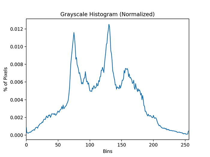
In Figure 1, we have plotted a histogram with 256 bins along the x-axis and the percentage of pixels falling into the given bins along the y-axis. Examining the histogram, note that there are three primary peaks.
The first peak in the histogram is around x=65 where we see a sharp spike in the number of pixels — clearly there is some sort of object in the image that has a very dark value.
We then see a much slower rising peak in the histogram, where we start to ascend around x=100 and finally end the descent around x=150. This region probably refers to a background region of the image.
Finally, we see there is a very large number of pixels in the range x=150 to x=175. It’s hard to say exactly what this region is, but it must dominate a large portion of the image.
Note: I’m intentionally not revealing which image I used to generate this histogram. I’m simply demonstrating my thought process as I look at a histogram. Being able to interpret and understand the data you are looking at, without necessarily knowing its source, is a good skill to have.
By simply examining the histogram of an image, you get a general understanding regarding the contrast, brightness, and intensity distribution. If this concept seems new or foreign to you, don’t worry — we’ll be examining more examples like this one later in this lesson.
Using OpenCV to compute histograms with the cv2.calcHist function

Let’s start building some histograms of our own.
We will be using the cv2.calcHist function to build our histograms. Before we get into any code examples, let’s quickly review the function:
cv2.calcHist(images, channels, mask, histSize, ranges)
images: This is the image that we want to compute a histogram for. Wrap it as a list:[myImage].channels: A list of indexes, where we specify the index of the channel we want to compute a histogram for. To compute a histogram of a grayscale image, the list would be[0]. To compute a histogram for all three red, green, and blue channels, the channels list would be[0, 1, 2].mask: Remember learning about masks in my Image Masking with OpenCV guide? Well, here we can supply a mask. If a mask is provided, a histogram will be computed for masked pixels only. If we do not have a mask or do not want to apply one, we can just provide a value ofNone.histSize: This is the number of bins we want to use when computing a histogram. Again, this is a list, one for each channel we are computing a histogram for. The bin sizes do not all have to be the same. Here is an example of 32 bins for each channel:[32, 32, 32].ranges: The range of possible pixel values. Normally, this is [0, 256] (that is not a typo — the ending range of thecv2.calcHistfunction is non-inclusive so you’ll want to provide a value of 256 rather than 255) for each channel, but if you are using a color space other than RGB [such as HSV], the ranges might be different.)
In the following sections, you’ll gain hands-on experience using the cv2.calcHist function to compute image histograms with OpenCV.
Configuring your development environment
To follow this guide, you need to have the OpenCV library installed on your system.
Luckily, OpenCV is pip-installable:
$ pip install opencv-contrib-python
If you need help configuring your development environment for OpenCV, I highly recommend that you read my pip install OpenCV guide — it will have you up and running in a matter of minutes.
Having problems configuring your development environment?
All that said, are you:
- Short on time?
- Learning on your employer’s administratively locked system?
- Wanting to skip the hassle of fighting with the command line, package managers, and virtual environments?
- Ready to run the code right now on your Windows, macOS, or Linux systems?
Then join PyImageSearch University today!
Gain access to Jupyter Notebooks for this tutorial and other PyImageSearch guides that are pre-configured to run on Google Colab’s ecosystem right in your web browser! No installation required.
And best of all, these Jupyter Notebooks will run on Windows, macOS, and Linux!
Project structure
Let’s get started by reviewing our project directory structure.
Start by accessing the “Downloads” section of this tutorial to retrieve the source code and example images. From there you’ll be presented with the following directory structure:
$ tree . --dirsfirst
.
├── beach.png
├── color_histograms.py
├── grayscale_histogram.py
└── histogram_with_mask.py

0 directories, 4 files
We have three Python scripts to review today:
grayscale_histogram.py: Demonstrates how to compute a pixel intensity histogram from an input, single channel, grayscale imagecolor_histograms.py: Shows out how to compute 1D (i.e., “flattened”), 2D, and 3D color histogramshistogram_with_mask.py: Demonstrates how to compute a histogram for only a masked region of an input image
Our single image, beach.png, serves as inputs to each of these three scripts.
Creating grayscale histograms with OpenCV
Let’s learn how to compute grayscale histograms using OpenCV. Open up the grayscale_histogram.py file in your project structure and we’ll get started:
# import the necessary packages
from matplotlib import pyplot as plt
import argparse
import cv2

# construct the argument parser and parse the arguments
ap = argparse.ArgumentParser()
ap.add_argument("-i", "--image", required=True,
	help="path to the image")
args = vars(ap.parse_args())
Lines 2-4 import our required Python packages. We’ll be using the pyplot module of matplotlib to plot our image histograms, argparse for command line arguments, and cv2 for our OpenCV bindings.
We only have a single command line argument to parse, --image, which is the path to our input image residing on disk.
Next, let’s load our input image from disk and convert it to grayscale:
# load the input image and convert it to grayscale
image = cv2.imread(args["image"])
image = cv2.cvtColor(image, cv2.COLOR_BGR2GRAY)
With the grayscale conversion complete we can use the cv2.calcHist function to compute our image histogram:
# compute a grayscale histogram
hist = cv2.calcHist([image], [0], None, [256], [0, 256])
Go ahead and match the arguments of the cv2.calcHist call with the function documentation in the “Using OpenCV to compute histograms with the cv2.calcHist function” section above.
We can see that our first parameter is the grayscale image. A grayscale image has only one channel, so we have a value of [0] for channels . We don’t have a mask, so we set the mask value to None. We will use 256 bins in our histogram, and the possible values range from 0 to 255.
With our image histogram computed we display the grayscale image on our screen and plot the unnormalized image histogram:
# matplotlib expects RGB images so convert and then display the image
# with matplotlib
plt.figure()
plt.axis("off")
plt.imshow(cv2.cvtColor(image, cv2.COLOR_GRAY2RGB))

# plot the histogram
plt.figure()
plt.title("Grayscale Histogram")
plt.xlabel("Bins")
plt.ylabel("# of Pixels")
plt.plot(hist)
plt.xlim([0, 256])
An unnormalized histogram counts the raw frequencies of the distribution. Consider counting the number of different colors of M&M’s in a bag. We would end up with an integer count for each of the individual colors.
On the other hand, what if I wanted the percentage of each of the colors?
Well, that’s easy enough to obtain! I would simply divide each of the integer counts by the total number of M&M’s in the bag. So instead of a raw frequency histogram, I would end up with a normalized histogram that counts the percentage of each color. And by definition, the sum of a normalized histogram is exactly 1.
So is there a reason why I would prefer a normalized histogram over an unnormalized one?
It turns out, there is. Let’s play a little thought experiment:
In this thought experiment we want to compare the histograms of two images. These images are identical in every way, shape, and form — with one exception. The first image is half the size of the second image.
And when we went to compare the histograms, while the shape of the distributions would look identical, we would notice that the pixel counts along the y-axis would be dramatically different. In fact, the y-axis counts for the first image would be exactly half the y-axis counts for the second image?
The reason for this being?
We were comparing raw frequency counts versus the percentage counts!
So with this in mind, let’s see how we can normalize a histogram and obtain our percentage counts for each pixel:
# normalize the histogram
hist /= hist.sum()

# plot the normalized histogram
plt.figure()
plt.title("Grayscale Histogram (Normalized)")
plt.xlabel("Bins")
plt.ylabel("% of Pixels")
plt.plot(hist)
plt.xlim([0, 256])
plt.show()
The normalization of the histogram takes only a single line of code, which we can see on Line 34: here we are simply dividing the raw frequency counts for each bin of the histogram by the sum of the counts — this leaves us with the percentage of each bin rather than the raw count of each bin.
We then plot the normalized histogram on Lines 37-43.
Grayscale histogram results
We are now ready to compute grayscale histograms with OpenCV!
Be sure to access the “Downloads” section of this guide to retrieve the source code and example image. From there, you can execute the following command:
$ python grayscale_histogram.py --image beach.png
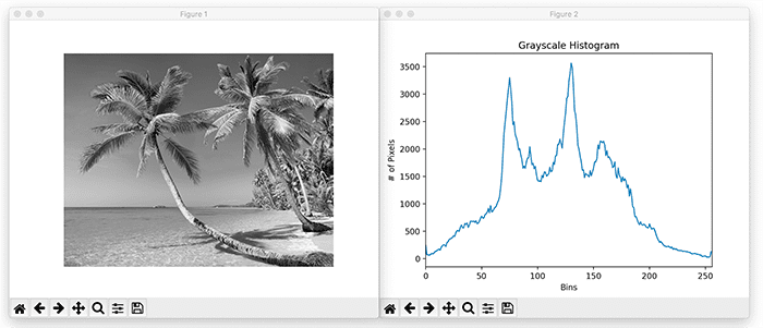
So, how do we interpret this histogram?
Well, the bins (0-255) are plotted on the x-axis. And the y-axis counts the number of pixels in each bin. The majority of the pixels fall in the range of roughly 60 to 180. Looking at both tails of the histogram, we can see that very few pixels fall in the range [0, 50] and [200, 255] — this implies that there are very few “black” and very few “white” pixels in the image.
Note that Figure 4 contains an unnormalized histogram, meaning that it contains the raw integer counts inside the bins.
If we instead want the percentage counts (such that when added all values sum to 1), we can inspect the normalized histogram:
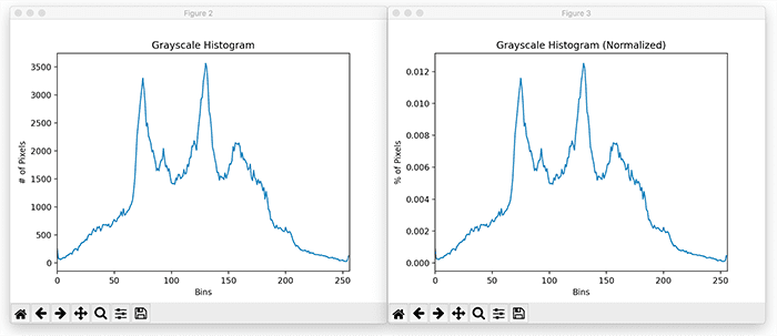
Now the bin counts are expressed as percentages rather than raw counts.
Depending on your application you may need either an unnormalized or normalized image histogram. I’ve demonstrated how to compute both types in this lesson, that way you have both methods available to you.
Creating color histograms with OpenCV
In the previous section, we explored grayscale histograms. Now let’s move on to computing a histogram for each channel of the image.
Open the color_histograms.py file in your project directory and we’ll get started:
# import the necessary packages
from matplotlib import pyplot as plt
import argparse
import imutils
import cv2

# construct the argument parser and parse the arguments
ap = argparse.ArgumentParser()
ap.add_argument("-i", "--image", required=True,
	help="path to the image")
args = vars(ap.parse_args())
Lines 2-5 import our required Python packages. Our imports are identical to that of grayscale_histogram.py, but with one exception — we’re now importing imutils which contains a handy opencv2matplotlib function which handles displaying RGB versus BGR images with matplotlib.
We then parse our command line arguments on Lines 8-11. We only need a single argument, --image, the path to our input image residing on disk.
Let’s now compute three histograms, one for each channel of the input RGB image:
# load the input image from disk
image = cv2.imread(args["image"])

# split the image into its respective channels, then initialize the
# tuple of channel names along with our figure for plotting
chans = cv2.split(image)
colors = ("b", "g", "r")
plt.figure()
plt.title("'Flattened' Color Histogram")
plt.xlabel("Bins")
plt.ylabel("# of Pixels")

# loop over the image channels
for (chan, color) in zip(chans, colors):
	# create a histogram for the current channel and plot it
	hist = cv2.calcHist([chan], [0], None, [256], [0, 256])
	plt.plot(hist, color=color)
	plt.xlim([0, 256])
Line 14 loads our image from disk. We then split the image into its respective BGR channels on Line 18.
Line 19 defines the list of channel names (strings) while Lines 20-23 initialize our matplotlib figure.
We then reach a for loop on Line 26. Here we start looping over each of the channels in the image.
Then, for each channel we compute a histogram on Line 28. The code is identical to that of computing a histogram for the grayscale image; however, we are doing it for each Red, Green, and Blue channel, allowing us to characterize the distribution of pixel intensities. We add our histogram to the plot on Line 29.
Let’s now look at computing a 2D histogram. Up until this point, we have computed a histogram for only one channel at a time. Now we move on to multi-dimensional histograms and take into consideration two channels at a time.
The way I like to explain multi-dimensional histograms is to use the word AND.
For example, we can ask a question such as:
- How many pixels have a Red value of 10 AND a Blue value of 30?
- How many pixels have a Green value of 200 AND a Red value of 130?
By using the conjunctive AND, we are able to construct multidimensional histograms.
It’s that simple. Let’s check out some code to automate the process of building a 2D histogram:
# create a new figure and then plot a 2D color histogram for the
# green and blue channels
fig = plt.figure()
ax = fig.add_subplot(131)
hist = cv2.calcHist([chans[1], chans[0]], [0, 1], None, [32, 32],
	[0, 256, 0, 256])
p = ax.imshow(hist, interpolation="nearest")
ax.set_title("2D Color Histogram for G and B")
plt.colorbar(p)

# plot a 2D color histogram for the green and red channels
ax = fig.add_subplot(132)
hist = cv2.calcHist([chans[1], chans[2]], [0, 1], None, [32, 32],
	[0, 256, 0, 256])
p = ax.imshow(hist, interpolation="nearest")
ax.set_title("2D Color Histogram for G and R")
plt.colorbar(p)

# plot a 2D color histogram for blue and red channels
ax = fig.add_subplot(133)
hist = cv2.calcHist([chans[0], chans[2]], [0, 1], None, [32, 32],
	[0, 256, 0, 256])
p = ax.imshow(hist, interpolation="nearest")
ax.set_title("2D Color Histogram for B and R")
plt.colorbar(p)

# finally, let's examine the dimensionality of one of the 2D
# histograms
print("2D histogram shape: {}, with {} values".format(
	hist.shape, hist.flatten().shape[0]))
Yes, this is a fair amount of code. But that’s only because we are computing a 2D color histogram for each combination of RGB channels: Red and Green, Red and Blue, and Green and Blue.
Now that we are working with multi-dimensional histograms, we need to keep in mind the number of bins we are using. In previous examples, I’ve used 256 bins for demonstration purposes.
However, if we used 256 bins for each dimension in a 2D histogram, our resulting histogram would have 65,536 separate pixel counts (since 256×256 = 65,536). Not only is this wasteful of resources, it’s not practical. Most applications use somewhere between 8 and 64 bins when computing multi-dimensional histograms. As Lines 36 and 37 show, I am now using 32 bins instead of 256.
The most important takeaway from this code can be seen by inspecting the first arguments to the cv2.calcHist function. Here we see that we are passing in a list of two channels: the Green and Blue channels. And that’s all there is to it.
So how is a 2D histogram stored in OpenCV? It’s a 2D NumPy array. Since I used 32 bins for each channel, I now have a 32×32 histogram.
As we’ll see when we run this script, our 2D histogram will have a dimensionality of 32×32 = 1,024 (Lines 60 and 61).
Using a 2D histogram takes into account two channels at a time. But what if we wanted to account for all three RGB channels? You guessed it. We’re now going to build a 3D histogram:
# our 2D histogram could only take into account 2 out of the 3
# channels in the image so now let's build a 3D color histogram
# (utilizing all channels) with 8 bins in each direction -- we
# can't plot the 3D histogram, but the theory is exactly like
# that of a 2D histogram, so we'll just show the shape of the
# histogram
hist = cv2.calcHist([image], [0, 1, 2],
	None, [8, 8, 8], [0, 256, 0, 256, 0, 256])
print("3D histogram shape: {}, with {} values".format(
	hist.shape, hist.flatten().shape[0]))
The code here is very simple — it’s just an extension from the 2D histogram code above. We are now computing an 8×8×8 histogram for each of the RGB channels. We can’t visualize this histogram, but we can see that the shape is indeed (8, 8, 8) with 512 values.
Finally, let’s display our original input image on our screen:
# display the original input image
plt.figure()
plt.axis("off")
plt.imshow(imutils.opencv2matplotlib(image))

# show our plots
plt.show()
The opencv2matplotlib convenience function from imutils is used for converting a BGR image to RGB. This handy method is also great if you ever work with Jupyter notebooks.
Color histogram results
We are now ready to compute color histograms with OpenCV!
Be sure to access the “Downloads” section of this tutorial to retrieve the source code and example image. From there you can execute the color_histograms.py script:
$ python color_histograms.py --image beach.png
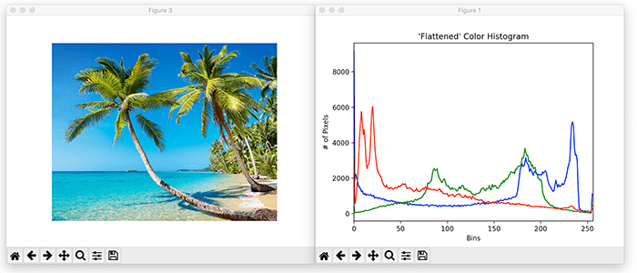
On the left, you can see our input image containing a tranquil beach scene. On the right, we have our “flattened” color histogram.
We see there is a sharp peak in the green histogram around bin 100. We see that most of the green pixels in the image are contained in the range [85, 200] — these regions are mid-range to light green from the green vegetation and trees in the beach image.
We also see a lot of lighter blue pixels in our image. Considering that we have both views of the crystal clear ocean and the cloudless blue sky, this should not be a surprise.
Let’s now visualize our 2D histograms:
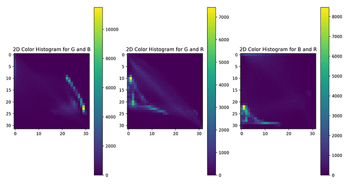
The first is a 2D color histogram for the Green and Blue channels, the second for Green and Red, and the third for Blue and Red. Shades of blue represent low pixel counts, whereas shades of red represent high pixel counts (i.e., peaks in the 2D histogram).
We tend to see many peaks in the Green and Blue histogram, where x=28 and y=27. This region corresponds to the green pixels of the vegetation and trees and the blue of the sky and ocean.
Furthermore, we can explore the shape of the image histogram via our command line output:
2D histogram shape: (32, 32), with 1024 values
3D histogram shape: (8, 8, 8), with 512 values
Each 2D histogram is 32×32. Multiplied out, that implies that means each histogram is 32×32 = 1024-d, implying that each histogram is represented by a total of 1,024 values.
Our 3D histogram on the other hand is 8×8×8, so when multiplied out, we see our 3D image histogram is represented by 512 values.
Computing image histograms for masked regions with OpenCV
So far we’ve learned how to compute histograms for the entirety of an input image? But what if you wanted to compute an image histogram for only a specific region of the input image?
For example, you may be building a computer vision application that automatically recognizes and matches clothing. You would first want to segment the clothing from the image. After that you would need to compute a color histogram to quantify the color distribution of the clothing … but you don’t want to include background pixels in the computation those pixels don’t belong to the clothing item itself.
So, what do you do in those situations?
Is it possible to compute a color histogram for only a specific region of an input image?
You bet it is.
Open histogram_with_mask.py in your project directory structure and I’ll show you how it’s done:
# import the necessary packages
from matplotlib import pyplot as plt
import numpy as np
import cv2
Lines 2-4 import our required Python packages. We’ll use matplotlib for plotting, NumPy for numerical array processing, and cv2 for our OpenCV bindings.
Let’s now define a convenience function, plot_histogram, which will wrap the majority of our matplotlib calls into a single, easy-to-use function:
def plot_histogram(image, title, mask=None):
	# split the image into its respective channels, then initialize
	# the tuple of channel names along with our figure for plotting
	chans = cv2.split(image)
	colors = ("b", "g", "r")
	plt.figure()
	plt.title(title)
	plt.xlabel("Bins")
	plt.ylabel("# of Pixels")

	# loop over the image channels
	for (chan, color) in zip(chans, colors):
		# create a histogram for the current channel and plot it
		hist = cv2.calcHist([chan], [0], mask, [256], [0, 256])
		plt.plot(hist, color=color)
		plt.xlim([0, 256])
On Line 6, we define plot_histogram. This function accepts three parameters: an image, the title of our plot, and a mask. The mask defaults to None if we do not have a mask for the image.
The body of our plot_histogram function simply computes a histogram for each channel in the image and plots it, just as in previous examples in this section; however, take note that we are now passing in the mask argument to cv2.calcHist.
In the event that we do have an input mask, we pass it in here, that way OpenCV knows to include only the masked pixels from the input image into the histogram construction.
With the plot_histogram function definition taken care of, we can move on to the rest of our script:
# load the beach image and plot a histogram for it
image = cv2.imread("beach.png")
plot_histogram(image, "Histogram for Original Image")
cv2.imshow("Original", image)
We start by loading our beach image from disk on Line 24, displaying it on screen on Line 25, and then plotting a color histogram for each channel of the beach image on Line 26.
Note that we are not passing in a mask here, so we are computing the color histogram for the entirety of the image.
Now, let’s learn how to compute a color histogram for only the masked region of an image:
# construct a mask for our image; our mask will be *black* for regions
# we want to *ignore* and *white* for regions we want to *examine*
mask = np.zeros(image.shape[:2], dtype="uint8")
cv2.rectangle(mask, (60, 290), (210, 390), 255, -1)
cv2.imshow("Mask", mask)

# display the masked region
masked = cv2.bitwise_and(image, image, mask=mask)
cv2.imshow("Applying the Mask", masked)

# compute a histogram for our image, but we'll only include pixels in
# the masked region
plot_histogram(image, "Histogram for Masked Image", mask=mask)

# show our plots
plt.show()
We define our mask as a NumPy array, with the same width and height as our beach image on Line 30. We then draw a white rectangle starting from point (60, 210) to point (290, 390) on Line 31.
This rectangle will serve as our mask — only pixels in our original image belonging to the masked region will be considered in the histogram computation.
Finally, we display the resulting plots on our screen (Line 43).
Masked histogram results
We are now ready to compute masked histograms for an image.
Be sure to access the “Downloads” section of this tutorial to retrieve the source code and example image. From there, you can execute the histogram_with_mask.py script:
$ python histogram_with_mask.py
To start, we display our original input image along with its corresponding channel histograms with no masking applied:
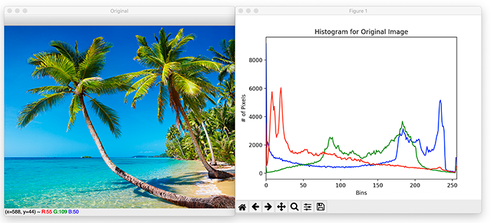
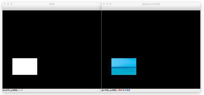
From there, we construct a rectangular mask and visualize the masked region of the image using a bitwise AND:
Finally, let’s compare the histogram for the entire image to the histogram computed from only the masked region of the image:
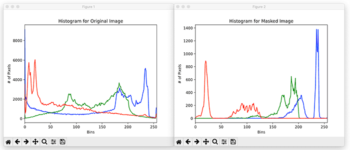
On the left, we have our histogram of the original image, whereas, on the right, we have our histogram for the masked image.
For the masked image, most red pixels fall in the range [10, 25], indicating that red pixels contribute very little to our image. This makes sense, since our ocean and sky are blue.
Green pixels are then present, but these are toward the lighter end of the distribution, which corresponds to the green foliage and trees.
Finally, our blue pixels fall in the brighter range and are obviously our blue ocean and sky.
Most importantly, compare our masked color histograms (right) to the unmasked color histograms (left) the above figure. Notice how dramatically different the color histograms are.
By utilizing masks, we are able to apply our computation only to the specific regions of the image that interest us — in this example, we simply wanted to examine the distribution of the blue sky and ocean.
What's next? We recommend PyImageSearch University.
86+ total classes • 115+ hours hours of on-demand code walkthrough videos • Last updated: May 2026
★★★★★ 4.84 (128 Ratings) • 16,000+ Students Enrolled
I strongly believe that if you had the right teacher you could master computer vision and deep learning.
Do you think learning computer vision and deep learning has to be time-consuming, overwhelming, and complicated? Or has to involve complex mathematics and equations? Or requires a degree in computer science?
That’s not the case.
All you need to master computer vision and deep learning is for someone to explain things to you in simple, intuitive terms. And that’s exactly what I do. My mission is to change education and how complex Artificial Intelligence topics are taught.
If you're serious about learning computer vision, your next stop should be PyImageSearch University, the most comprehensive computer vision, deep learning, and OpenCV course online today. Here you’ll learn how to successfully and confidently apply computer vision to your work, research, and projects. Join me in computer vision mastery.
Inside PyImageSearch University you'll find:
- ✓ 86+ courses on essential computer vision, deep learning, and OpenCV topics
- ✓ 86 Certificates of Completion
- ✓ 115+ hours hours of on-demand video
- ✓ Brand new courses released regularly, ensuring you can keep up with state-of-the-art techniques
- ✓ Pre-configured Jupyter Notebooks in Google Colab
- ✓ Run all code examples in your web browser — works on Windows, macOS, and Linux (no dev environment configuration required!)
- ✓ Access to centralized code repos for all 540+ tutorials on PyImageSearch
- ✓ Easy one-click downloads for code, datasets, pre-trained models, etc.
- ✓ Access on mobile, laptop, desktop, etc.
Summary
In this tutorial, you learned all about image histograms and how to compute them using OpenCV and the cv2.calcHist function.
Histograms are very simple, but are very powerful tools to have. They are used extensively for thresholding, color correction, and even image features! Make sure you have a good grasp of histograms, you’ll be certainly using them in the future.
To download the source code to this post (and be notified when future tutorials are published here on PyImageSearch), simply enter your email address in the form below!

Download the Source Code and FREE 17-page Resource Guide
Enter your email address below to get a .zip of the code and a FREE 17-page Resource Guide on Computer Vision, OpenCV, and Deep Learning. Inside you'll find my hand-picked tutorials, books, courses, and libraries to help you master CV and DL!


Comment section
Hey, Adrian Rosebrock here, author and creator of PyImageSearch. While I love hearing from readers, a couple years ago I made the tough decision to no longer offer 1:1 help over blog post comments.
At the time I was receiving 200+ emails per day and another 100+ blog post comments. I simply did not have the time to moderate and respond to them all, and the sheer volume of requests was taking a toll on me.
Instead, my goal is to do the most good for the computer vision, deep learning, and OpenCV community at large by focusing my time on authoring high-quality blog posts, tutorials, and books/courses.
If you need help learning computer vision and deep learning, I suggest you refer to my full catalog of books and courses — they have helped tens of thousands of developers, students, and researchers just like yourself learn Computer Vision, Deep Learning, and OpenCV.
Click here to browse my full catalog.