Object detection: Bounding box regression with Keras, TensorFlow, and Deep Learning

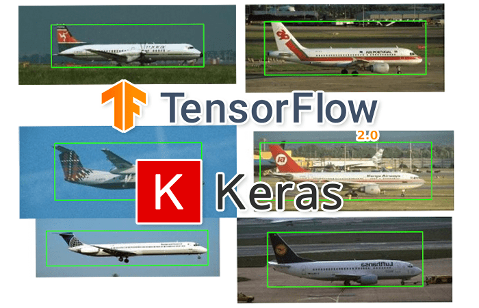
In this tutorial you will learn how to train a custom deep learning model to perform object detection via bounding box regression with Keras and TensorFlow.

A dataset with images annotated with bounding boxes and class labels is essential for understanding bounding box regression for object detection. It helps to train models that not only recognize objects but also accurately predict their location in the image.

Roboflow has free tools for each stage of the computer vision pipeline that will streamline your workflows and supercharge your productivity.

Sign up or Log in to your Roboflow account to access state of the art dataset libaries and revolutionize your computer vision pipeline.

You can start by choosing your own datasets or using our PyimageSearch’s assorted library of useful datasets.

Bring data in any of 40+ formats to Roboflow, train using any state-of-the-art model architectures, deploy across multiple platforms (API, NVIDIA, browser, iOS, etc), and connect to applications or 3rd party tools.

Today’s tutorial is inspired by a message I received from PyImageSearch reader Kyle:

Hi Adrian,

Many thanks for your four-part series of tutorials on region proposal object detectors. It helped me understand the basics of how R-CNN object detectors work.

But I’m a bit confused by the term “bounding box regression.” What does that mean? How does bounding box regression work? And how does bounding box regression predict locations of objects in images?

Great questions, Kyle.

Basic R-CNN object detectors, such as the ones we covered on the PyImageSearch blog, rely on the concept of region proposal generators.

These region proposal algorithms (e.g., Selective Search) examine an input image and then identify where a potential object could be. Keep in mind that they have absolutely no idea if an object exists in a given location, just that the area of the image looks interesting and warrants further inspection.

In the classic implementation of Girshick et al.’s R-CNN, these region proposals were used to extract output features from a pre-trained CNN (minus the fully-connected layer head) and then were fed into an SVM for final classification. In this implementation the location from the regional proposal was treated as the bounding box, while the SVM produced the class label for the bounding box region.

Essentially, the original R-CNN architecture didn’t actually “learn” how to detect bounding boxes — it was not end-to-end trainable (future iterations, such as Faster R-CNN, actually were end-to-end trainable).

But that raises the questions:

• What if we wanted to train an end-to-end object detector?
• Is it possible to construct a CNN architecture that can output bounding box coordinates, that way we can actually train the model to make better object detector predictions?
• And if so, how do we go about training such a model?

The key to all those questions lies in the concept of bounding box regression, which is exactly what we’ll be covering today. By the end of this tutorial, you’ll have an end-to-end trainable object detector capable of producing both bounding box predictions and class label predictions for objects in an image.

To learn how to perform object detection via bounding box regression with Keras, TensorFlow, and Deep Learning, just keep reading.

Object detection: Bounding box regression with Keras, TensorFlow, and Deep Learning

In the first part of this tutorial, we’ll briefly discuss the concept of bounding box regression and how it can be used to train an end-to-end object detector.

We’ll then discuss the dataset we’ll be using to train our bounding box regressor.

From there, we’ll review our directory structure for the project, along with a simple Python configuration file (since our implementation spans multiple files). Given our configuration file, we’ll be able to implement a script to actually train our object detection model via bounding box regression with Keras and TensorFlow.

With our model trained, we’ll implement a second Python script, this one to handle inference (i.e., making object detection predictions) on new input images.

Let’s get started!

What is bounding box regression?

We are all likely familiar with the concept of image classification via deep neural networks. When performing image classification, we:

1. Present an input image to the CNN
2. Perform a forward pass through the CNN
3. Output a vector with N elements, where N is the total number of class labels
4. Select the class label with the largest probability as our final predicted class label

Fundamentally, we can think of image classification as predicting a class label.

But unfortunately, that type of model doesn’t translate to object detection. It would be impossible for us to construct a class label for every possible combination of (x, y)-coordinate bounding boxes in an input image.

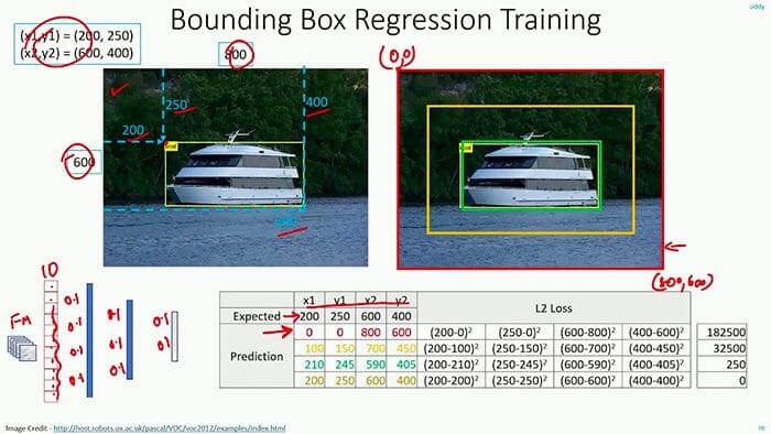
Instead, we need to rely on a different type of machine learning model called regression. Unlike classification, which produces a label, regression enables us to predict continuous values.

Typically, regression models are applied to problems such as:

• Predicting the price of a home (which we actually did in this tutorial)
• Forecasting the stock market
• Determining the rate of a disease spreading through a population
• etc.

The point here is that a regression model’s output isn’t limited to being discretized into “bins” like a classification model is (remember, a classification model can only output a class label, nothing more).

Instead, a regression model can output any real value in a specific range.

Typically, we scale the output range of values to [0, 1] during training and then scale the outputs back after prediction (if needed).

In order to perform bounding box regression for object detection, all we need to do is adjust our network architecture:

1. At the head of the network, place a fully-connected layer with four neurons, corresponding to the top-left and bottom-right (x, y)-coordinates, respectively.
2. Given that four-neuron layer, implement a sigmoid activation function such that the outputs are returned in the range [0, 1].
3. Train the model using a loss function such as mean-squared error or mean-absolute error on training data that consists of (1) the input images and (2) the bounding box of the object in the image.

After training, we can present an input image to our bounding box regressor network. Our network will then perform a forward pass and then actually predict the output bounding box coordinates of the object.

We’ll be covering object detection via bounding box regression for a single class in this tutorial, but next week we’ll extend it to multi-class object detection as well.

Our object detection and bounding box regression dataset

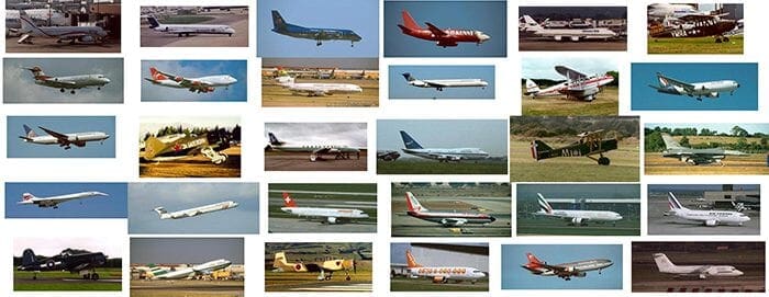
The example dataset we are using here today is a subset of the CALTECH-101 dataset, which can be used to train object detection models.

Specifically, we’ll be using the airplane class consisting of 800 images and the corresponding bounding box coordinates of the airplanes in the image. I have included a subset of the airplane example images in Figure 2.

Our goal is to train an object detector capable of accurately predicting the bounding box coordinates of airplanes in the input images.

Note: There’s no need to download the full dataset from CALTECH-101’s website. I’ve included the subset of airplane images, including a CSV file of the bounding boxes, in the “Downloads” section associated with this tutorial.

Configuring your development environment

To configure your system for this tutorial, I recommend following either of these tutorials:

• How to install TensorFlow 2.0 on Ubuntu
• How to install TensorFlow 2.0 on macOS

Either tutorial will help you configure your system with all the necessary software for this blog post in a convenient Python virtual environment.

That said, are you:

• Short on time?
• Learning on your employer’s administratively locked laptop?
• Wanting to skip the hassle of fighting with package managers, bash/ZSH profiles, and virtual environments?
• Ready to run the code right now (and experiment with it to your heart’s content)?

Then join PyImageSearch Plus today! Gain access to PyImageSearch tutorial Jupyter Notebooks that run on Google’s Colab ecosystem in your browser — no installation required!

Project structure

Go ahead and grab the .zip from the “Downloads” section of this tutorial. Inside, you’ll find the subset of data as well as our project files:

$ tree --dirsfirst --filelimit 10
.
├── dataset
│   ├── images [800 entries]
│   └── airplanes.csv
├── output
│   ├── detector.h5
│   ├── plot.png
│   └── test_images.txt
├── pyimagesearch
│   ├── __init__.py
│   └── config.py
├── predict.py
└── train.py

4 directories, 8 files

Creating our configuration file

Before we can implement our bounding box regression training script, we need to create a simple Python configuration file that will store variables reused across our training and prediction script, including image paths, model paths, etc.

Open up the config.py file, and let’s take a peek:

# import the necessary packages
import os

# define the base path to the input dataset and then use it to derive
# the path to the images directory and annotation CSV file
BASE_PATH = "dataset"
IMAGES_PATH = os.path.sep.join([BASE_PATH, "images"])
ANNOTS_PATH = os.path.sep.join([BASE_PATH, "airplanes.csv"])

# define the path to the base output directory
BASE_OUTPUT = "output"

# define the path to the output serialized model, model training plot,
# and testing image filenames
MODEL_PATH = os.path.sep.join([BASE_OUTPUT, "detector.h5"])
PLOT_PATH = os.path.sep.join([BASE_OUTPUT, "plot.png"])
TEST_FILENAMES = os.path.sep.join([BASE_OUTPUT, "test_images.txt"])

# initialize our initial learning rate, number of epochs to train
# for, and the batch size
INIT_LR = 1e-4
NUM_EPOCHS = 25
BATCH_SIZE = 32

Our deep learning hyperparameters include the initial learning rate, number of epochs, and batch size. These parameters are in one convenient place so that you can keep track of your experimental inputs and results.

Implementing our bounding box regression training script with Keras and TensorFlow

With our configuration file implemented, we can move to creating our bounding box regression training script.

This script will be responsible for:

1. Loading our airplane training data from disk (i.e., both class labels and bounding box coordinates)
2. Loading VGG16 from disk (pre-trained on ImageNet), removing the fully-connected classification layer head from the network, and inserting our bounding box regression layer head
3. Fine-tuning the bounding box regression layer head on our training data

I’ll be assuming that you’re already comfortable with modifying the architecture of a network and fine-tuning it.

If you are not already comfortable with this concept, I suggest you read the article linked above before continuing.

Bounding box regression is a concept best explained through code, so open up the train.py file in your project directory, and let’s get to work:

# import the necessary packages
from pyimagesearch import config
from tensorflow.keras.applications import VGG16
from tensorflow.keras.layers import Flatten
from tensorflow.keras.layers import Dense
from tensorflow.keras.layers import Input
from tensorflow.keras.models import Model
from tensorflow.keras.optimizers import Adam
from tensorflow.keras.preprocessing.image import img_to_array
from tensorflow.keras.preprocessing.image import load_img
from sklearn.model_selection import train_test_split
import matplotlib.pyplot as plt
import numpy as np
import cv2
import os

Our training script begins with a selection of imports. These include:

• config: The configuration file we developed in the previous section consisting of paths and hyperparameters
• VGG16: The CNN architecture to serve as the base network for our fine tuning approach
• tf.keras: Imports from TensorFlow/Keras consisting of layer types, optimizers, and image loading/preprocessing routines
• train_test_split: Scikit-learn’s convenience utility for slicing our network into training and testing subsets
• matplotlib: Python’s de facto plotting package
• numpy: Python’s standard numerical processing library
• cv2: OpenCV

Again, you’ll need to follow the “Configuring your development environment” section to ensure that you have all the necessary software installed, or elect to run this script in a Jupyter Notebook.

Now that our environment is ready and packages are imported, let’s work with our data:

# load the contents of the CSV annotations file
print("[INFO] loading dataset...")
rows = open(config.ANNOTS_PATH).read().strip().split("\n")

# initialize the list of data (images), our target output predictions
# (bounding box coordinates), along with the filenames of the
# individual images
data = []
targets = []
filenames = []

Here, we load our bounding box annotations CSV data (Line 19). Each record in the file consists of an image filename and any object bounding boxes associated with that image.

We then make three list initializations:

• data: Will soon hold all of our images
• targets: Will soon hold all of our predictions and bounding box coordinates
• filenames: The filenames associated with the actual image data

These are three separate lists that correspond to one another. We’ll now begin a loop that seeks to populate the lists from the CSV data:

# loop over the rows
for row in rows:
	# break the row into the filename and bounding box coordinates
	row = row.split(",")
	(filename, startX, startY, endX, endY) = row

Looping over all rows in the CSV file (Line 29), our first step is to unpack the particular entry’s filename and bounding box coordinates (Lines 31 and 32).

To get a feel for the CSV data, let’s take a peek inside:

image_0001.jpg,49,30,349,137
image_0002.jpg,59,35,342,153
image_0003.jpg,47,36,331,135
image_0004.jpg,47,24,342,141
image_0005.jpg,48,18,339,146
image_0006.jpg,48,24,344,126
image_0007.jpg,49,23,344,122
image_0008.jpg,51,29,344,119
image_0009.jpg,50,29,344,137
image_0010.jpg,55,32,335,106

As you can see, each row consists of five elements:

1. Filename
2. Starting x-coordinate
3. Starting y-coordinate
4. Ending x-coordinate
5. Ending y-coordinate

These are exactly the values that Line 32 of our script has unpacked into convenience variables for this loop iteration.

Still working through our loop, next we’ll load an image:

	# derive the path to the input image, load the image (in OpenCV
	# format), and grab its dimensions
	imagePath = os.path.sep.join([config.IMAGES_PATH, filename])
	image = cv2.imread(imagePath)
	(h, w) = image.shape[:2]

	# scale the bounding box coordinates relative to the spatial
	# dimensions of the input image
	startX = float(startX) / w
	startY = float(startY) / h
	endX = float(endX) / w
	endY = float(endY) / h

Let’s wrap up our loop:

	# load the image and preprocess it
	image = load_img(imagePath, target_size=(224, 224))
	image = img_to_array(image)

	# update our list of data, targets, and filenames
	data.append(image)
	targets.append((startX, startY, endX, endY))
	filenames.append(filename)

Now that we’ve loaded the data, let’s partition it for training:

# convert the data and targets to NumPy arrays, scaling the input
# pixel intensities from the range [0, 255] to [0, 1]
data = np.array(data, dtype="float32") / 255.0
targets = np.array(targets, dtype="float32")

# partition the data into training and testing splits using 90% of
# the data for training and the remaining 10% for testing
split = train_test_split(data, targets, filenames, test_size=0.10,
	random_state=42)

# unpack the data split
(trainImages, testImages) = split[:2]
(trainTargets, testTargets) = split[2:4]
(trainFilenames, testFilenames) = split[4:]

# write the testing filenames to disk so that we can use then
# when evaluating/testing our bounding box regressor
print("[INFO] saving testing filenames...")
f = open(config.TEST_FILENAMES, "w")
f.write("\n".join(testFilenames))
f.close()

Here we:

# load the VGG16 network, ensuring the head FC layers are left off
vgg = VGG16(weights="imagenet", include_top=False,
	input_tensor=Input(shape=(224, 224, 3)))

# freeze all VGG layers so they will *not* be updated during the
# training process
vgg.trainable = False

# flatten the max-pooling output of VGG
flatten = vgg.output
flatten = Flatten()(flatten)

# construct a fully-connected layer header to output the predicted
# bounding box coordinates
bboxHead = Dense(128, activation="relu")(flatten)
bboxHead = Dense(64, activation="relu")(bboxHead)
bboxHead = Dense(32, activation="relu")(bboxHead)
bboxHead = Dense(4, activation="sigmoid")(bboxHead)

# construct the model we will fine-tune for bounding box regression
model = Model(inputs=vgg.input, outputs=bboxHead)

Accomplishing fine-tuning is a four-step process:

1. Load VGG16 with pre-trained ImageNet weights, chopping off the old fully-connected classification layer head (Lines 79 and 80).
2. Freeze all layers in the body of the VGG16 network (Line 84).
3. Perform network surgery by constructing a new fully-connected layer head that will output four values corresponding to the top-left and bottom-right bounding box coordinates of an object in an image (Lines 87-95).
4. Finish network surgery by suturing the new trainable head (bounding box regression layers) to the existing frozen body (Line 98).

And now let’s train (i.e., fine-tune) our newly formed beast:

# initialize the optimizer, compile the model, and show the model
# summary
opt = Adam(lr=config.INIT_LR)
model.compile(loss="mse", optimizer=opt)
print(model.summary())

# train the network for bounding box regression
print("[INFO] training bounding box regressor...")
H = model.fit(
	trainImages, trainTargets,
	validation_data=(testImages, testTargets),
	batch_size=config.BATCH_SIZE,
	epochs=config.NUM_EPOCHS,
	verbose=1)

# serialize the model to disk
print("[INFO] saving object detector model...")
model.save(config.MODEL_PATH, save_format="h5")

# plot the model training history
N = config.NUM_EPOCHS
plt.style.use("ggplot")
plt.figure()
plt.plot(np.arange(0, N), H.history["loss"], label="train_loss")
plt.plot(np.arange(0, N), H.history["val_loss"], label="val_loss")
plt.title("Bounding Box Regression Loss on Training Set")
plt.xlabel("Epoch #")
plt.ylabel("Loss")
plt.legend(loc="lower left")
plt.savefig(config.PLOT_PATH)

Training our basic bounding box regressor and object detector

With our bounding box regression network implemented, let’s move on to training it.

Start by using the “Downloads” section of this tutorial to download the source code and example airplane dataset.

From there, open up a terminal, and execute the following command:

$ python train.py
[INFO] loading dataset...
[INFO] saving testing filenames...

Our script starts by loading our airplane dataset from disk.

We then construct our training/testing split and then save the filenames of the images inside the testing set to disk (so we can use them later on when making predictions with our trained network).

From there, our training script outputs the model summary of our VGG16 network with the bounding box regression head:

Model: "model"
_________________________________________________________________
Layer (type)                 Output Shape              Param #
=================================================================
input_1 (InputLayer)         [(None, 224, 224, 3)]     0
_________________________________________________________________
block1_conv1 (Conv2D)        (None, 224, 224, 64)      1792
_________________________________________________________________
block1_conv2 (Conv2D)        (None, 224, 224, 64)      36928
_________________________________________________________________
block1_pool (MaxPooling2D)   (None, 112, 112, 64)      0
_________________________________________________________________
block2_conv1 (Conv2D)        (None, 112, 112, 128)     73856
_________________________________________________________________
block2_conv2 (Conv2D)        (None, 112, 112, 128)     147584
_________________________________________________________________
block2_pool (MaxPooling2D)   (None, 56, 56, 128)       0
_________________________________________________________________
block3_conv1 (Conv2D)        (None, 56, 56, 256)       295168
_________________________________________________________________
block3_conv2 (Conv2D)        (None, 56, 56, 256)       590080
_________________________________________________________________
block3_conv3 (Conv2D)        (None, 56, 56, 256)       590080
_________________________________________________________________
block3_pool (MaxPooling2D)   (None, 28, 28, 256)       0
_________________________________________________________________
block4_conv1 (Conv2D)        (None, 28, 28, 512)       1180160
_________________________________________________________________
block4_conv2 (Conv2D)        (None, 28, 28, 512)       2359808
_________________________________________________________________
block4_conv3 (Conv2D)        (None, 28, 28, 512)       2359808
_________________________________________________________________
block4_pool (MaxPooling2D)   (None, 14, 14, 512)       0
_________________________________________________________________
block5_conv1 (Conv2D)        (None, 14, 14, 512)       2359808
_________________________________________________________________
block5_conv2 (Conv2D)        (None, 14, 14, 512)       2359808
_________________________________________________________________
block5_conv3 (Conv2D)        (None, 14, 14, 512)       2359808
_________________________________________________________________
block5_pool (MaxPooling2D)   (None, 7, 7, 512)         0
_________________________________________________________________
flatten (Flatten)            (None, 25088)             0
_________________________________________________________________
dense (Dense)                (None, 128)               3211392
_________________________________________________________________
dense_1 (Dense)              (None, 64)                8256
_________________________________________________________________
dense_2 (Dense)              (None, 32)                2080
_________________________________________________________________
dense_3 (Dense)              (None, 4)                 132
=================================================================
Total params: 17,936,548
Trainable params: 3,221,860
Non-trainable params: 14,714,688

Pay attention to the layers following block5_pool (MaxPooling2D) — these layers correspond to our bounding box regression layer head.

When trained, these layers will learn how to predict the bounding box (x, y)-coordinates of an object in an image!

Next comes our actual training process:

[INFO] training bounding box regressor...
Epoch 1/25
23/23 [==============================] - 37s 2s/step - loss: 0.0239 - val_loss: 0.0014
Epoch 2/25
23/23 [==============================] - 38s 2s/step - loss: 0.0014 - val_loss: 8.7668e-04
Epoch 3/25
23/23 [==============================] - 36s 2s/step - loss: 9.1919e-04 - val_loss: 7.5377e-04
Epoch 4/25
23/23 [==============================] - 37s 2s/step - loss: 7.1202e-04 - val_loss: 8.2668e-04
Epoch 5/25
23/23 [==============================] - 36s 2s/step - loss: 6.1626e-04 - val_loss: 6.4373e-04
...
Epoch 20/25
23/23 [==============================] - 37s 2s/step - loss: 6.9272e-05 - val_loss: 5.6152e-04
Epoch 21/25
23/23 [==============================] - 36s 2s/step - loss: 6.3215e-05 - val_loss: 5.4341e-04
Epoch 22/25
23/23 [==============================] - 37s 2s/step - loss: 5.7234e-05 - val_loss: 5.5000e-04
Epoch 23/25
23/23 [==============================] - 37s 2s/step - loss: 5.4265e-05 - val_loss: 5.5932e-04
Epoch 24/25
23/23 [==============================] - 37s 2s/step - loss: 4.5151e-05 - val_loss: 5.4348e-04
Epoch 25/25
23/23 [==============================] - 37s 2s/step - loss: 4.0826e-05 - val_loss: 5.3977e-04
[INFO] saving object detector model...

After training the bounding box regressor, the following training history plot is produced:

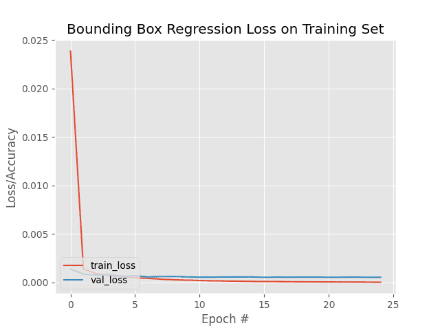
Our object detection model starts off with high loss but is able to descend into areas of lower loss during the training process (i.e., where the model learns how to make better bounding box predictions).

After training is complete, your output directory should contain the following files:

$ ls output/
detector.h5	plot.png	test_images.txt

The plot.png file contains our training history plot while test_images.txt contains the filenames of the images in our testing set (which we’ll make predictions on later in this tutorial).

Implementing our bounding box predictor with Keras and TensorFlow

At this point we have our bounding box predictor serialized to disk — but how do we use that model to detect objects in input images?

We’ll be answering that question in this section.

Open up a new file, name it predict.py, and insert the following code:

# import the necessary packages
from pyimagesearch import config
from tensorflow.keras.preprocessing.image import img_to_array
from tensorflow.keras.preprocessing.image import load_img
from tensorflow.keras.models import load_model
import numpy as np
import mimetypes
import argparse
import imutils
import cv2
import os

At this point, you should recognize all imports except imutils (my computer vision convenience package) and potentially mimetypes (built into Python; can recognize filetypes from filenames and URLs).

Let’s parse command line arguments:

# construct the argument parser and parse the arguments
ap = argparse.ArgumentParser()
ap.add_argument("-i", "--input", required=True,
	help="path to input image/text file of image filenames")
args = vars(ap.parse_args())

# determine the input file type, but assume that we're working with
# single input image
filetype = mimetypes.guess_type(args["input"])[0]
imagePaths = [args["input"]]

# if the file type is a text file, then we need to process *multiple*
# images
if "text/plain" == filetype:
	# load the filenames in our testing file and initialize our list
	# of image paths
	filenames = open(args["input"]).read().strip().split("\n")
	imagePaths = []

	# loop over the filenames
	for f in filenames:
		# construct the full path to the image filename and then
		# update our image paths list
		p = os.path.sep.join([config.IMAGES_PATH, f])
		imagePaths.append(p)

1. Default: Our imagePaths consist of one lone image path from --input (Line 22).
2. Text File: If the conditional/check for text filetype on Line 26 holds True, then we override and populate our imagePaths from all the filenames (one per line) in the --input text file (Lines 29-37).

Given one or more testing images, let’s start performing bounding box regression with our deep learning TensorFlow/Keras model:

# load our trained bounding box regressor from disk
print("[INFO] loading object detector...")
model = load_model(config.MODEL_PATH)

# loop over the images that we'll be testing using our bounding box
# regression model
for imagePath in imagePaths:
	# load the input image (in Keras format) from disk and preprocess
	# it, scaling the pixel intensities to the range [0, 1]
	image = load_img(imagePath, target_size=(224, 224))
	image = img_to_array(image) / 255.0
	image = np.expand_dims(image, axis=0)

Upon loading our model (Line 41), we begin looping over images (Line 45). Inside, we first load and preprocess the image in the exact same way we did for training. This includes:

• Resizing the image to 224×224 pixels (Line 48)
• Converting to array format and scaling pixels to the range [0, 1] (Line 49)
• Adding a batch dimension (Line 50)

And from there, we can perform bounding box regression inference and annotate the result:

	# make bounding box predictions on the input image
	preds = model.predict(image)[0]
	(startX, startY, endX, endY) = preds

	# load the input image (in OpenCV format), resize it such that it
	# fits on our screen, and grab its dimensions
	image = cv2.imread(imagePath)
	image = imutils.resize(image, width=600)
	(h, w) = image.shape[:2]

	# scale the predicted bounding box coordinates based on the image
	# dimensions
	startX = int(startX * w)
	startY = int(startY * h)
	endX = int(endX * w)
	endY = int(endY * h)

	# draw the predicted bounding box on the image
	cv2.rectangle(image, (startX, startY), (endX, endY),
		(0, 255, 0), 2)

	# show the output image
	cv2.imshow("Output", image)
	cv2.waitKey(0)

Line 53 makes bounding box predictions on the input image. Notice that preds contains our bounding box prediction’s (x, y)-coordinates; we unpack these values for convenience via Line 54.

Now we have everything we need for annotation. To annotate the bounding box on the image, we simply:

• Load the original Image from disk with OpenCV and resize it while maintaining aspect ratio (Lines 58 and 59)
• Scale the predicted bounding box coordinates from the range [0, 1] to the range [0, w] and [0, h] where w and h are the width and height of the input image (Lines 60-67)
• Draw the scaled bounding box (Lines 70 and 71)

Finally, we show the output on the screen. Pressing a key cycles through the loop, displaying results one-by-one until all testing images have been exhausted (Lines 74 and 75).

Great job! Let’s inspect our results in the next section.

Bounding box regression and object detection results with Keras and TensorFlow

We are now ready to put our bounding box regression object detection model to the test!

Make sure you’ve used the “Downloads” section of this tutorial to download the source code, image dataset, and pre-trained object detection model.

From there, let’s try applying object detection to a single input image:

$ python predict.py --input dataset/images/image_0697.jpg
[INFO] loading object detector...

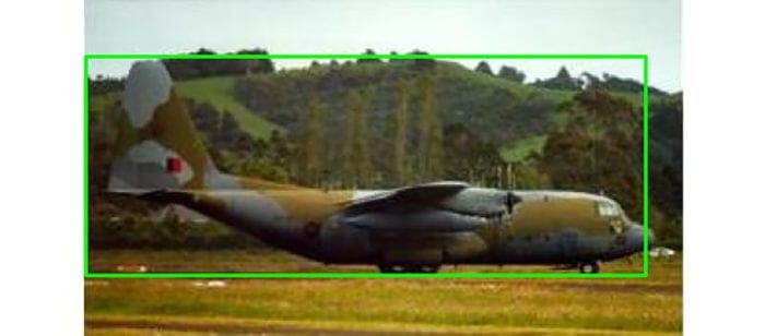
As you can see, our bounding box regressor has correctly localized the airplane in the input image, demonstrating that our object detection model actually learned how to predict bounding box coordinates just from the input image!

Next, let’s apply the bounding box regressor to every image in the test set by supplying the path to the test_images.txt file as the --input command line argument:

$ python predict.py --input output/test_images.txt
[INFO] loading object detector...

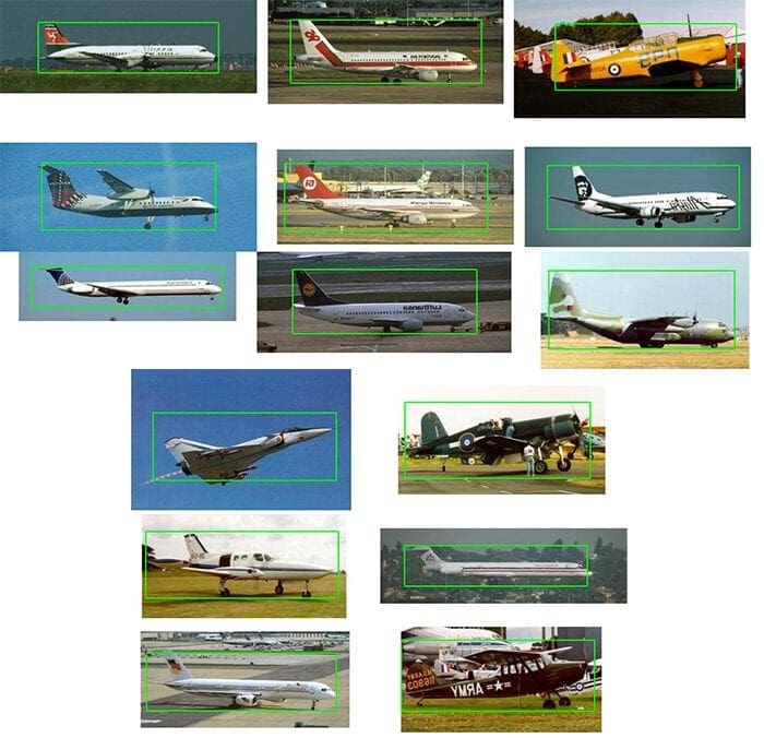
As Figure 6 shows, our object detection model is doing a great job of predicting the location of airplanes in our input images!

Limitations

At this point we’ve successfully trained a model for bounding box regression — but an obvious limitation of this architecture is that it can only predict bounding boxes for a single class.

What if we wanted to perform multi-class object detection where we not only have an “airplanes” class but also “motorcycles,” “cars,” and “trucks?”

Is multi-class object detection even possible with bounding box regression?

You bet it is — and I’ll be covering that very topic in next week’s tutorial. We’ll learn how multi-class object detection requires changes to the bounding box regression architecture (hint: two branches in our CNN) and train such a model. Stay tuned!

Summary

In this tutorial you learned how to train an end-to-end object detector with bounding box regression.

To accomplish this task we utilized the Keras and TensorFlow deep learning libraries.

Unlike classification models, which output only class labels, regression models are capable of producing real-valued outputs.

Typical applications of regression models include predicting the price of homes, forecasting the stock market, and predicting the rate at which a disease spreads through a region.

However, regression models are not limited to price forecasting or disease spreading — we can use them for object detection as well!

The trick is to update your CNN architecture to:

1. Place a fully-connected layer with four neurons (top-left and bottom-right bounding box coordinates) at the head of the network
2. Put a sigmoid activation function on that layer (such that output values lie in the range [0, 1])
3. Train your model by providing (1) the input image and (2) the target bounding boxes of the object in the image
4. Subsequently, train your model using mean-squared error, mean-absolute error, etc.

The final result is an end-to-end trainable object detector, similar to the one we built today!

You’ll note that our model can only predict one type of class label though — how can we extend our implementation to handle multiple labels?

Is that possible?

You bet it is — stay tuned next week for part two in this series!

To download the source code to this post (and be notified when future tutorials are published here on PyImageSearch), simply enter your email address in the form below!