Multiprocessing with OpenCV and Python

In this tutorial, you will learn how to use multiprocessing with OpenCV and Python to perform feature extraction. You’ll learn how to use multiprocessing with OpenCV to parallelize feature extraction across the system bus, including all processors and cores on your computer.

Today’s tutorial is inspired by PyImageSearch reader, Abigail.

Abigail writes:

Hey Adrian, I just read your tutorial on image hashing with OpenCV and really enjoyed it.

I’m trying to apply image hashing to my research project at the university.

They have provided me with a dataset of ~7.5 million images. I used your code to perform image hashing but it’s taking a long time to process the entire dataset.

Is there anything I can do to speedup the process?

Abigail asks a great question.

The image hashing post she is referring to is singled threaded, meaning that only one core of the processor is being utilized — if we switch to using multiple threads/processes we can dramatically speed up the hashing process.

But how do we actually utilize multiprocessing with OpenCV and Python?

I’ll show you in the rest of this tutorial.

To learn how to use multiprocessing with OpenCV and Python, just keep reading.

Multiprocessing with OpenCV and Python

In the first part of this tutorial, we’ll discuss single-threaded vs. multi-threaded applications, including why we may choose to use multiprocessing with OpenCV to speed up the processing of a given dataset.

I’ll also discuss why immediately jumping to Big Data algorithms, tools, and paradigms (such as Hadoop and MapReduce) is the wrong decision — instead, you should parallelize across the system bus first.

From there we’ll implement our Python and OpenCV multiprocessing functions to facilitate processing a large dataset quickly and easily.

Finally, we’ll put all the pieces together and compare how long it takes to process our dataset:

1. With only a single core of a processor
2. And distributing the load across all cores of the processor

Let’s get started!

Why use multiprocessing for processing a dataset of images?

The vast majority of projects and applications you have implemented are (very likely) single-threaded.

When you launch your Python project, the python binary launches a Python interpreter (i.e., the “Python process”).

How the actual Python process itself is assigned to a CPU core is dependent on how the operating system handles (1) process scheduling and (2) assigning system vs. user threads.

There are entire books dedicated to multiprocessing, operating systems, and how processes are scheduled, assigned, removed, deleted, etc. via the OS; however, for the sake of simplicity, let’s assume:

1. We launch our Python script.
2. The operating system assigns the Python program to a single core of the processor.
3. The OS then allows the Python script to run on the processor core until completion.

That’s all fine and good — but we are only utilizing a small amount of our true processing power.

To see how we’re underutilizing our processor, consider the following image:

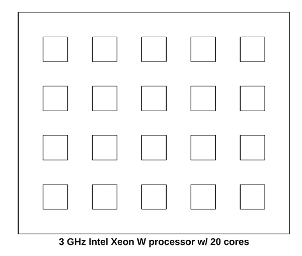
This figure is meant to visualize the 3 GHz Intel Xeon W on my iMac Pro — note how the processor has a total of 20 cores.

Now, let’s assume we launch our Python script. The operating system will assign the process to a single one of those cores:

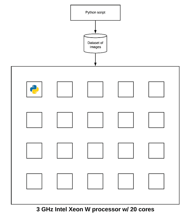
The Python script will then run to completion.

But do you see the problem here?

We are only using 5% of our true processing power!

Thus, to speed up our Python script we can utilize multiprocessing. Under the hood, Python’s multiprocessing package spins up a new python process for each core of the processor. Each python process is independent and separate from the others (i.e., there are no shared variables, memory, etc.).

We then assign a portion of the dataset processing workload to each individual python process:

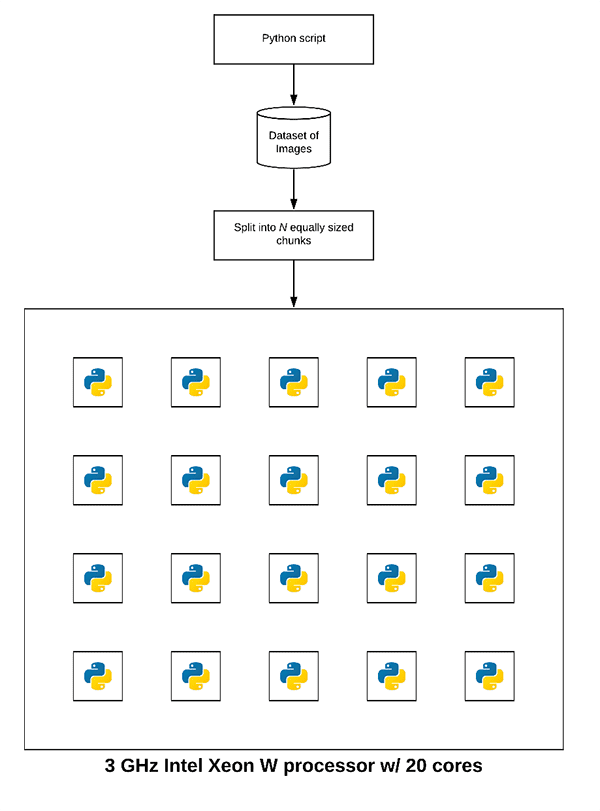
Notice how each process is assigned a small chunk of the dataset.

Each process independently chews on the subset of the dataset assigned to it until the entire dataset has been processed.

Now, instead of using just a single core of our processor, we are using all cores!

Note: Keep in mind that this example is a bit of a simplification. The OS will manage process assignment as there are more processes than just your Python script running on your system. Some cores may be responsible for more than one Python process, other cores no Python processes, and remaining cores OS/system routines.

Why not use Hadoop, MapReduce, and other Big Data tools?

Your first thought when trying to parallelize processing of a large dataset would be to apply Big Data tools, algorithms, and paradigms such as Hadoop and MapReduce — but this would be a BIG mistake.

The golden rule when working with large datasets is to:

1. Parallelize across your system bus first.
2. And if performance/throughput is not sufficient, then, and only then, start parallelizing across multiple machines (including Hadoop, MapReduce, etc.).

The single biggest multiprocessing mistake I see computer scientists make is to immediately jump into Big Data tools.

Don’t do that.

Instead, spread the dataset processing across your system bus first.

If you’re not getting the throughput speed you want on your system bus only then should you consider parallelizing across multiple machines and bringing in Big Data tools.

If you find yourself in need of Hadoop/MapReduce, enroll in the PyImageSearch Gurus course to learn about high-throughput Python + OpenCV image processing using Hadoop’s Streaming API!

Our example dataset

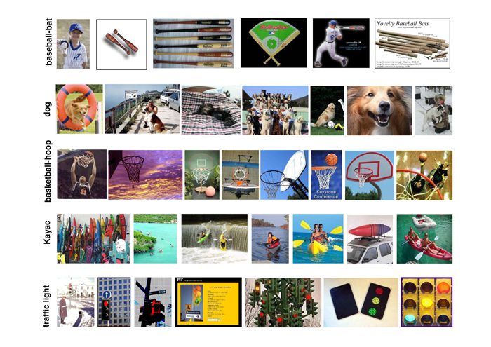
The dataset we’ll be using for our multiprocessing and OpenCV example is CALTECH-101, the same dataset we use when building an image hashing search engine.

The dataset consists of 9,144 images.

We’ll be using multiprocessing to spread out the image hashing extraction across all cores of our processor.

You may download the CALTECH-101 dataset from their official webpage or you can use the following wget command:

$ wget http://www.vision.caltech.edu/Image_Datasets/Caltech101/101_ObjectCategories.tar.gz
$ tar xvzf 101_ObjectCategories.tar.gz

Project structure

Let’s inspect our project structure:

$ tree --dirsfirst --filelimit 10
.
├── pyimagesearch
│   ├── __init__.py
│   └── parallel_hashing.py
├── 101_ObjectCategories [9,144 images] 
├── temp_output
└── extract.py

Inside the pyimagesearch module is our parallel_hashing.py helper script. This script contains our hashing function, chunking function, and our process_images workhorse.

The 101_ObjectCatories/ directory contains 101 subdirectories of images from CALTECH-101 (downloaded via the previous section).

A number of intermediate files will be temporarily stored in the temp_output/ folder.

The heart of our multiprocessing lies in extract.py . This script includes our pre-multiprocessing overhead, parallelization across the system bus, and post-multprocessing overhead.

Our multiprocessing helper functions

Before we can utilize multiprocessing with OpenCV to speedup our dataset processing, let’s first implement our set of helper utilities used to facilitate multiprocessing.

Open up the parallel_hashing.py file in your directory structure and insert the following code:

# import the necessary packages
import numpy as np
import pickle
import cv2

def dhash(image, hashSize=8):
	# convert the image to grayscale
	gray = cv2.cvtColor(image, cv2.COLOR_BGR2GRAY)

	# resize the input image, adding a single column (width) so we
	# can compute the horizontal gradient
	resized = cv2.resize(gray, (hashSize + 1, hashSize))

	# compute the (relative) horizontal gradient between adjacent
	# column pixels
	diff = resized[:, 1:] > resized[:, :-1]

	# convert the difference image to a hash
	return sum([2 ** i for (i, v) in enumerate(diff.flatten()) if v])

We begin by importing NumPy, OpenCV, and pickle (Lines 2-5).

From there, we define our difference hashing function, dhash . There are a number of image hashing algorithms, but one of the most popular ones is called the difference hash, which includes four steps:

1. Step #1: Convert the input image to grayscale (Line 8).
2. Step #2: Resize the image to fixed dimensions, N + 1 x N, ignoring aspect ratio. Typically we set N=8 or N=16. We use N + 1 for the number of rows so that we can compute the difference (hence “difference hash”) between adjacent pixels in the image (Line 12).
3. Step #3: Compute the difference. If we set N=8 then we have 9 pixels per row and 8 pixels per column. We can then compute the difference between adjacent column pixels, yielding 8 differences. 8 rows of 8 differences (i.e., 8×8) results in 64 values (Line 16).
4. Step #4: Finally, we can build the hash. In practice all we actually need to perform is a “greater than” operation comparing the columns, yielding binary values. These 64 binary values are compacted into an integer, forming our final hash (Line 19).

Typically, image hashing algorithms are used to find near-duplicate images in a large dataset.

For a full review of difference hashing be sure to review the following two blog posts:

• Building an Image Hashing Search Engine with VP-Trees and OpenCV
• Image hashing with OpenCV and Python

Next, let’s look at the convert_hash function:

def convert_hash(h):
	# convert the hash to NumPy's 64-bit float and then back to
	# Python's built in int
	return int(np.array(h, dtype="float64"))

When I first wrote the code for the image hashing search engine tutorial, I found that the VP-Tree implementation internally converts points to a NumPy 64-bit float. That would be okay; however, hashes need to be integers and if we convert them to 64-bit floats, they become an unhashable data type. To overcome the limitation of the VP-Tree implementation, I came up with the convert_hash hack:

• We accept an input hash, h .
• That hash is then converted to a NumPy 64-bit float.
• And that NumPy float is then converted back to Python’s built-in integer data type.

This hack ensures that hashes are represented consistently throughout the hashing, indexing, and searching process.

In order to leverage multiprocessing, we first need to chunk our dataset into N equally sized chunks (one chunk per core of the processor).

Let’s define our chunk generator now:

def chunk(l, n):
	# loop over the list in n-sized chunks
	for i in range(0, len(l), n):
		# yield the current n-sized chunk to the calling function
		yield l[i: i + n]

The chunk generator accepts two parameters:

• l: List of elements (in this case, file paths).
• n: Number of N-sized chunks to generate.

Inside the function, we loop over list l and yield N-sized chunks to the calling function.

We’re finally to the workhorse of our multiprocessing implementation — the process_images function:

def process_images(payload):
	# display the process ID for debugging and initialize the hashes
	# dictionary
	print("[INFO] starting process {}".format(payload["id"]))
	hashes = {}

	# loop over the image paths
	for imagePath in payload["input_paths"]:
		# load the input image, compute the hash, and conver it
		image = cv2.imread(imagePath)
		h = dhash(image)
		h = convert_hash(h)

		# update the hashes dictionary
		l = hashes.get(h, [])
		l.append(imagePath)
		hashes[h] = l

	# serialize the hashes dictionary to disk using the supplied
	# output path
	print("[INFO] process {} serializing hashes".format(payload["id"]))
	f = open(payload["output_path"], "wb")
	f.write(pickle.dumps(hashes))
	f.close()

Inside the separate extract.py script, we’ll use Python’s multiprocessing library to launch a dedicated Python process, assign it to a specific core of the processor, and then run the process_images function on that specific core.

The process_images function works like this:

• It accepts a payload as an input (Line 32). The payload is assumed to be a Python dictionary but can actually be any datatype provided that we can pickle and unpickle it.
• Initializes the hashes dictionary (Line 36).
• Loops over input image paths in the payload (Line 39). In the loop, we load each image, extract the hash, and update hashes dictionary (Lines 41-48).
• Finally, we write the hashes to disk as a .pickle file (Lines 53-55).

For the purposes of this blog post we are utilizing multiprocessing to facilitate faster image hashing of an input dataset; however, you should use this function as a template for your own dataset processing.

You should easily swap in keypoint detection/local invariant feature extraction, color channel statistics, Local Binary Patterns, etc. From there, you may take this function an modify it for your own needs.

Implementing the OpenCV and multiprocessing script

Now that our utility methods are implemented, let’s create the multiprocessing driver script.

This script will be responsible for:

1. Grabbing all image paths in our input dataset.
2. Splitting the image paths into N equally sized chunks (where N is the total number of processes we wish to utilize).
3. Using multiprocessing, Pool, and map to call the process_images function on each core of the processor.
4. Grab the results from each independent process and combine them.

If you need to review Python’s multiprocessing module, be sure to refer to the docs.

Let’s see how we can implement our OpenCV and multiprocessing script. Open up the extract.py file and insert the following code:

# import the necessary packages
from pyimagesearch.parallel_hashing import process_images
from pyimagesearch.parallel_hashing import chunk
from multiprocessing import Pool
from multiprocessing import cpu_count
from imutils import paths
import numpy as np
import argparse
import pickle
import os

Lines 2-10 import our packages, modules, and functions:

• From our custom parallel_hashing file, we import both our process_images and chunk functions.
• To accommodate parallel processing we’ll use Pythons multiprocessing module. Specifically, we import Pool (to construct a processing pool) and cpu_count (to get a count of the number of available CPUs/cores if the --procs command line argument is not supplied).

All of our multiprocessing setup code must be in the main thread of execution:

# check to see if this is the main thread of execution
if __name__ == "__main__":
	# construct the argument parser and parse the arguments
	ap = argparse.ArgumentParser()
	ap.add_argument("-i", "--images", required=True, type=str,
		help="path to input directory of images")
	ap.add_argument("-o", "--output", required=True, type=str,
		help="path to output directory to store intermediate files")
	ap.add_argument("-a", "--hashes", required=True, type=str,
		help="path to output hashes dictionary")
	ap.add_argument("-p", "--procs", type=int, default=-1,
		help="# of processes to spin up")
	args = vars(ap.parse_args())

Line 13 ensures we are inside the main thread of execution. This helps prevent multiprocessing bugs, especially on Windows operating systems.

Lines 15-24 parse four command line arguments:

• --images : The path to the input images directory.
• --output : The path to the output directory to store intermediate files.
• --hashes : The path to the output hashes dictionary in .pickle format.
• --procs : The number of processes to launch for multiprocessing.

With our command line arguments parsed and ready to go, now we’ll (1) determine the number of concurrent processes to launch, and (2) prepare our image paths (a bit of pre-multiprocessing overhead):

	# determine the number of concurrent processes to launch when
	# distributing the load across the system, then create the list
	# of process IDs
	procs = args["procs"] if args["procs"] > 0 else cpu_count()
	procIDs = list(range(0, procs))

	# grab the paths to the input images, then determine the number
	# of images each process will handle
	print("[INFO] grabbing image paths...")
	allImagePaths = sorted(list(paths.list_images(args["images"])))
	numImagesPerProc = len(allImagePaths) / float(procs)
	numImagesPerProc = int(np.ceil(numImagesPerProc))

	# chunk the image paths into N (approximately) equal sets, one
	# set of image paths for each individual process
	chunkedPaths = list(chunk(allImagePaths, numImagesPerProc))

Line 29 determines the total number of concurrent processes we’ll be launching, while Line 30 assigns each process an ID number. By default, we’ll utilize all CPUs/cores on our system.

Line 35 grabs paths to the input images in our dataset.

Lines 36 and 37 determine the total number of images per process by dividing the number of image paths by the number of processes and taking the ceiling to ensure we use an integer value from here forward.

Line 41 utilizes our chunk function to create a list of N equally-sized lists of image paths. We will be mapping each of these chunks to an independent process.

Let’s prepare our payloads to assign to each process (our final pre-multiprocessing overhead):

	# initialize the list of payloads
	payloads = []

	# loop over the set chunked image paths
	for (i, imagePaths) in enumerate(chunkedPaths):
		# construct the path to the output intermediary file for the
		# current process
		outputPath = os.path.sep.join([args["output"],
			"proc_{}.pickle".format(i)])

		# construct a dictionary of data for the payload, then add it
		# to the payloads list
		data = {
			"id": i,
			"input_paths": imagePaths,
			"output_path": outputPath
		}
		payloads.append(data)

Line 44 initializes the payloads list. Each payload will consist of data containing:

1. An ID
2. A list of input paths
3. An output path to an intermediate file

Line 47 begins a loop over our chunked image paths. Inside the loop, we specify the intermediary output file path (which will store the respective image hashes for that specific chunk of image paths) while naming it carefully with the process ID in the filename (Lines 50 and 51).

To finish the loop, we append our data — a dictionary consisting of the (1) ID, i , (2) input imagePaths , and (3) outputPath (Lines 55-60).

This next block is where we distribute processing of the dataset across our system bus:

	# construct and launch the processing pool
	print("[INFO] launching pool using {} processes...".format(procs))
	pool = Pool(processes=procs)
	pool.map(process_images, payloads)

	# close the pool and wait for all processes to finish
	print("[INFO] waiting for processes to finish...")
	pool.close()
	pool.join()
	print("[INFO] multiprocessing complete")

The Pool class creates the Python processes/interpreters on each respective core of the processor (Line 64).

Calling map takes the payloads list and then calls process_images on each core, distributing the payloads to each core (Lines 65).

We’ll then close the pool from accepting new jobs and wait for the multiprocessing to complete (Lines 69 and 70).

The final step (post-multiprocessing overhead) is to take our intermediate hashes and construct the final combined hashes.

	# initialize our *combined* hashes dictionary (i.e., will combine
	# the results of each pickled/serialized dictionary into a
	# *single* dictionary
	print("[INFO] combining hashes...")
	hashes = {}

	# loop over all pickle files in the output directory
	for p in paths.list_files(args["output"], validExts=(".pickle"),):
		# load the contents of the dictionary
		data = pickle.loads(open(p, "rb").read())

		# loop over the hashes and image paths in the dictionary
		for (tempH, tempPaths) in data.items():
			# grab all image paths with the current hash, add in the
			# image paths for the current pickle file, and then
			# update our hashes dictionary
			imagePaths = hashes.get(tempH, [])
			imagePaths.extend(tempPaths)
			hashes[tempH] = imagePaths

	# serialize the hashes dictionary to disk
	print("[INFO] serializing hashes...")
	f = open(args["hashes"], "wb")
	f.write(pickle.dumps(hashes))
	f.close()

Line 77 initializes the hashes dictionary to hold our combined hashes which we will populate from each of the intermediary files.

Lines 80-91 populate the combined hashes dictionary. To do so, we loop over all intermediate .pickle files (i.e., one .pickle file for each individual process). Inside the loop, we (1) read the hashes and associated imagePaths from the data, and (2) update the hashes dictionary.

Finally, Lines 94-97 serialize the hashes to disk. We could use the serialized hashes to construct a VP-Tree and search for near-duplicate images in a separate script at this point.

Note: You could update the code to delete the temporary .pickle files from your system; however, I left that as an implementation decision to you, the reader.

OpenCV and multiprocessing results

Let’s put our OpenCV and multiprocessing methods to the test. Make sure you’ve:

1. Used the “Downloads” section of this tutorial to download the source code.
2. Downloaded the CALTECH-101 dataset using the instructions in the “Our example dataset” section above.

To start, let’s test how long it takes to process our dataset of 9,144 images using only a single core:

$ time python extract.py --images 101_ObjectCategories --output temp_output \
	--hashes hashes.pickle --procs 1
[INFO] grabbing image paths...
[INFO] launching pool using 1 processes...
[INFO] starting process 0
[INFO] process 0 serializing hashes
[INFO] waiting for processes to finish...
[INFO] multiprocessing complete
[INFO] combining hashes...
[INFO] serializing hashes...

real	0m9.576s
user	0m7.857s
sys		0m1.489s

Utilizing only a single process (single core of our processor) required 9.576 seconds to process the entire image dataset.

Now, let’s try using all 20 processes (which could be mapped to all 20 cores of my processor):

$ time python extract.py --images ~/Desktop/101_ObjectCategories \
	--output temp_output --hashes hashes.pickle 
[INFO] grabbing image paths...
[INFO] launching pool using 20 processes...
[INFO] starting process 0
[INFO] starting process 1
[INFO] starting process 2
[INFO] starting process 3
[INFO] starting process 4
[INFO] starting process 5
[INFO] starting process 6
[INFO] starting process 7
[INFO] starting process 8
[INFO] starting process 9
[INFO] starting process 10
[INFO] starting process 11
[INFO] starting process 12
[INFO] starting process 13
[INFO] starting process 14
[INFO] starting process 15
[INFO] starting process 16
[INFO] starting process 17
[INFO] starting process 18
[INFO] starting process 19
[INFO] process 3 serializing hashes
[INFO] process 4 serializing hashes
[INFO] process 6 serializing hashes
[INFO] process 8 serializing hashes
[INFO] process 5 serializing hashes
[INFO] process 19 serializing hashes
[INFO] process 11 serializing hashes
[INFO] process 10 serializing hashes
[INFO] process 16 serializing hashes
[INFO] process 14 serializing hashes
[INFO] process 15 serializing hashes
[INFO] process 18 serializing hashes
[INFO] process 7 serializing hashes
[INFO] process 17 serializing hashes
[INFO] process 12 serializing hashes
[INFO] process 9 serializing hashes
[INFO] process 13 serializing hashes
[INFO] process 2 serializing hashes
[INFO] process 1 serializing hashes
[INFO] process 0 serializing hashes
[INFO] waiting for processes to finish...
[INFO] multiprocessing complete
[INFO] combining hashes...
[INFO] serializing hashes...

real	0m1.508s
user	0m12.785s
sys		0m1.361s

By distributing the image hashing load across all 20 cores of my processor I was able to reduce the time it took to process the dataset from 9.576 seconds down to 1.508 seconds — that’s a reduction of over 535%!

But wait, if we used 20 cores, shouldn’t the total processing time be approximately 9.576 / 20 = 0.4788 seconds?

Well, not quite, for a few reasons:

1. First, we’re performing a lot of I/O operations. Each cv2.imread call results in I/O overhead. The hashing algorithm itself is also very simple. If our algorithm were truly CPU bound, versus I/O bound, the speedup factor would be even better.
2. Secondly, multiprocessing is not a “free” operation. There are overhead function calls, both at the Python level and operating system level, that prevent us from seeing a true 20x speedup.

Can all computer vision and OpenCV algorithms be made parallel with multiprocessing?

The short answer is no, not all algorithms can be made parallel and distributed to all cores of a processor — some algorithms are simply single threaded in nature.

Furthermore, you cannot use the multiprocessing library to speedup compiled OpenCV routines like cv2.GaussianBlur, cv2.Canny, or any of the deep neural network routines in the cv2.dnn package.

Those routines, as well as all other cv2.* functions are pre-compiled C/C++ functions — Python’s multiprocessing library will have no impact on them whatsoever.

Instead, if you are interested in how to speedup those functions, be sure to look into OpenCL, Threading Building Blocks (TBB), NEON, and VFPv3.

Additionally, if you are working with the Raspberry Pi you should read this tutorial on how to optimize your OpenCV install.

I’m also including additional OpenCV optimizations inside my book, Raspberry Pi for Computer Vision.

Summary

In this tutorial you learned how to utilize multiprocessing with OpenCV and Python.

Specifically, we learned how to use Python’s built-in multiprocessing library along with the Pool and map methods to parallelize and distribute processing across all processors and all cores of the processors.

The end result is a massive 535% speedup in the time it took to process our dataset of images.

We examined multiprocessing with OpenCV through indexing a dataset of images for building an image hashing search engine; however, you can modify/implement your own process_images function to include your own functionality.

My personal suggestion would be to use the process_images function as a template when building your own multiprocessing and OpenCV applications.

I hope you enjoyed this tutorial!

If you would like to see more multiprocessing and OpenCV optimization tutorials in the future please leave a comment below and let me know.

To download the source code to this post, and be notified when future tutorials are published here on PyImageSearch, just enter your email address in the form below!