I’m going to start today’s blog post by asking a series of questions which will then be addressed later in the tutorial:
- What are image convolutions?
- What do they do?
- Why do we use them?
- How do we apply them?
- And what role do convolutions play in deep learning?

The word “convolution” sounds like a fancy, complicated term — but it’s really not. In fact, if you’ve ever worked with computer vision, image processing, or OpenCV before, you’ve already applied convolutions, whether you realize it or not!
Ever apply blurring or smoothing? Yep, that’s a convolution.
What about edge detection? Yup, convolution.
Have you opened Photoshop or GIMP to sharpen an image? You guessed it — convolution.
Convolutions are one of the most critical, fundamental building-blocks in computer vision and image processing. But the term itself tends to scare people off — in fact, on the the surface, the word even appears to have a negative connotation.
Trust me, convolutions are anything but scary. They’re actually quite easy to understand.
In reality, an (image) convolution is simply an element-wise multiplication of two matrices followed by a sum.
Seriously. That’s it. You just learned what convolution is:
- Take two matrices (which both have the same dimensions).
- Multiply them, element-by-element (i.e., not the dot-product, just a simple multiplication).
- Sum the elements together.
To understand more about convolutions, why we use them, how to apply them, and the overall role they play in deep learning + image classification, be sure to keep reading this post.
Convolutions with OpenCV and Python
Think of it this way — an image is just a multi-dimensional matrix. Our image has a width (# of columns) and a height (# of rows), just like a matrix.
But unlike the traditional matrices you may have worked with back in grade school, images also have a depth to them — the number of channels in the image. For a standard RGB image, we have a depth of 3 — one channel for each of the Red, Green, and Blue channels, respectively.
Given this knowledge, we can think of an image as a big matrix and kernel or convolutional matrix as a tiny matrix that is used for blurring, sharpening, edge detection, and other image processing functions.
Essentially, this tiny kernel sits on top of the big image and slides from left-to-right and top-to-bottom, applying a mathematical operation (i.e., a convolution) at each (x, y)-coordinate of the original image.
It’s normal to hand-define kernels to obtain various image processing functions. In fact, you might already be familiar with blurring (average smoothing, Gaussian smoothing, median smoothing, etc.), edge detection (Laplacian, Sobel, Scharr, Prewitt, etc.), and sharpening — all of these operations are forms of hand-defined kernels that are specifically designed to perform a particular function.
So that raises the question, is there a way to automatically learn these types of filters? And even use these filters for image classification and object detection?
You bet there is.
But before we get there, we need to understand kernels and convolutions a bit more.
Kernels
Again, let’s think of an image as a big matrix and a kernel as tiny matrix (at least in respect to the original “big matrix” image):
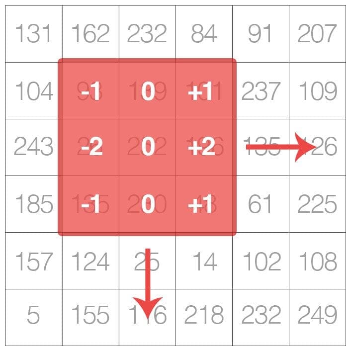
As the figure above demonstrates, we are sliding the kernel from left-to-right and top-to-bottom along the original image.
At each (x, y)-coordinate of the original image, we stop and examine the neighborhood of pixels located at the center of the image kernel. We then take this neighborhood of pixels, convolve them with the kernel, and obtain a single output value. This output value is then stored in the output image at the same (x, y)-coordinates as the center of the kernel.
If this sounds confusing, no worries, we’ll be reviewing an example in the “Understanding Image Convolutions” section later in this blog post.
But before we dive into an example, let’s first take a look at what a kernel looks like:

Above we have defined a square 3 x 3 kernel (any guesses on what this kernel is used for?)
Kernels can be an arbitrary size of M x N pixels, provided that both M and N are odd integers.
Note: Most kernels you’ll typically see are actually square N x N matrices.
We use an odd kernel size to ensure there is a valid integer (x, y)-coordinate at the center of the image:
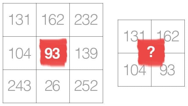
On the left, we have a 3 x 3 matrix. The center of the matrix is obviously located at x=1, y=1 where the top-left corner of the matrix is used as the origin and our coordinates are zero-indexed.
But on the right, we have a 2 x 2 matrix. The center of this matrix would be located at x=0.5, y=0.5. But as we know, without applying interpolation, there is no such thing as pixel location (0.5, 0.5) — our pixel coordinates must be integers! This reasoning is exactly why we use odd kernel sizes — to always ensure there is a valid (x, y)-coordinate at the center of the kernel.
Understanding Image Convolutions
Now that we have discussed the basics of kernels, let’s talk about a mathematical term called convolution.
In image processing, a convolution requires three components:
- An input image.
- A kernel matrix that we are going to apply to the input image.
- An output image to store the output of the input image convolved with the kernel.
Convolution itself is actually very easy. All we need to do is:
- Select an (x, y)-coordinate from the original image.
- Place the center of the kernel at this (x, y)-coordinate.
- Take the element-wise multiplication of the input image region and the kernel, then sum up the values of these multiplication operations into a single value. The sum of these multiplications is called the kernel output.
- Use the same (x, y)-coordinates from Step #1, but this time, store the kernel output in the same (x, y)-location as the output image.
Below you can find an example of convolving (denoted mathematically as the “*” operator) a 3 x 3 region of an image with a 3 x 3 kernel used for blurring:

Therefore,

After applying this convolution, we would set the pixel located at the coordinate (i, j) of the output image O to O_i,j = 126.
That’s all there is to it!
Convolution is simply the sum of element-wise matrix multiplication between the kernel and neighborhood that the kernel covers of the input image.
Implementing Convolutions with OpenCV and Python
That was fun discussing kernels and convolutions — but now let’s move on to looking at some actual code to ensure you understand how kernels and convolutions are implemented. This source code will also help you understand how to apply convolutions to images.
Open up a new file, name it convolutions.py , and let’s get to work:
# import the necessary packages
from skimage.exposure import rescale_intensity
import numpy as np
import argparse
import cv2
We start on Lines 2-5 by importing our required Python packages. You should already have NumPy and OpenCV installed on your system, but you might not have scikit-image installed. To install scikit-image, just use pip :
$ pip install -U scikit-image
Next, we can start defining our custom convolve method:
def convolve(image, kernel):
	# grab the spatial dimensions of the image, along with
	# the spatial dimensions of the kernel
	(iH, iW) = image.shape[:2]
	(kH, kW) = kernel.shape[:2]

	# allocate memory for the output image, taking care to
	# "pad" the borders of the input image so the spatial
	# size (i.e., width and height) are not reduced
	pad = (kW - 1) // 2
	image = cv2.copyMakeBorder(image, pad, pad, pad, pad,
		cv2.BORDER_REPLICATE)
	output = np.zeros((iH, iW), dtype="float32")
The convolve function requires two parameters: the (grayscale) image that we want to convolve with the kernel .
Given both our image and kernel (which we presume to be NumPy arrays), we then determine the spatial dimensions (i.e., width and height) of each (Lines 10 and 11).
Before we continue, it’s important to understand that the process of “sliding” a convolutional matrix across an image, applying the convolution, and then storing the output will actually decrease the spatial dimensions of our output image.
Why is this?
Recall that we “center” our computation around the center (x, y)-coordinate of the input image that the kernel is currently positioned over. This implies there is no such thing as “center” pixels for pixels that fall along the border of the image. The decrease in spatial dimension is simply a side effect of applying convolutions to images. Sometimes this effect is desirable and other times its not, it simply depends on your application.
However, in most cases, we want our output image to have the same dimensions as our input image. To ensure this, we apply padding (Lines 16-19). Here we are simply replicating the pixels along the border of the image, such that the output image will match the dimensions of the input image.
Other padding methods exist, including zero padding (filling the borders with zeros — very common when building Convolutional Neural Networks) and wrap around (where the border pixels are determined by examining the opposite end of the image). In most cases, you’ll see either replicate or zero padding.
We are now ready to apply the actual convolution to our image:
	# loop over the input image, "sliding" the kernel across
	# each (x, y)-coordinate from left-to-right and top to
	# bottom
	for y in np.arange(pad, iH + pad):
		for x in np.arange(pad, iW + pad):
			# extract the ROI of the image by extracting the
			# *center* region of the current (x, y)-coordinates
			# dimensions
			roi = image[y - pad:y + pad + 1, x - pad:x + pad + 1]

			# perform the actual convolution by taking the
			# element-wise multiplicate between the ROI and
			# the kernel, then summing the matrix
			k = (roi * kernel).sum()

			# store the convolved value in the output (x,y)-
			# coordinate of the output image
			output[y - pad, x - pad] = k
Lines 24 and 25 loop over our image , “sliding” the kernel from left-to-right and top-to-bottom 1 pixel at a time.
Line 29 extracts the Region of Interest (ROI) from the image using NumPy array slicing. The roi will be centered around the current (x, y)-coordinates of the image . The roi will also have the same size as our kernel , which is critical for the next step.
Convolution is performed on Line 34 by taking the element-wise multiplication between the roi and kernel , followed by summing the entries in the matrix.
The output value k is then stored in the output array at the same (x, y)-coordinates (relative to the input image).
We can now finish up our convolve method:
	# rescale the output image to be in the range [0, 255]
	output = rescale_intensity(output, in_range=(0, 255))
	output = (output * 255).astype("uint8")

	# return the output image
	return output
When working with images, we typically deal with pixel values falling in the range [0, 255]. However, when applying convolutions, we can easily obtain values that fall outside this range.
In order to bring our output image back into the range [0, 255], we apply the rescale_intensity function of scikit-image (Line 41). We also convert our image back to an unsigned 8-bit integer data type on Line 42 (previously, the output image was a floating point type in order to handle pixel values outside the range [0, 255]).
Finally, the output image is returned to the calling function on Line 45.
Now that we’ve defined our convolve function, let’s move on to the driver portion of the script. This section of our program will handle parsing command line arguments, defining a series of kernels we are going to apply to our image, and then displaying the output results:
# construct the argument parse and parse the arguments
ap = argparse.ArgumentParser()
ap.add_argument("-i", "--image", required=True,
	help="path to the input image")
args = vars(ap.parse_args())

# construct average blurring kernels used to smooth an image
smallBlur = np.ones((7, 7), dtype="float") * (1.0 / (7 * 7))
largeBlur = np.ones((21, 21), dtype="float") * (1.0 / (21 * 21))

# construct a sharpening filter
sharpen = np.array((
	[0, -1, 0],
	[-1, 5, -1],
	[0, -1, 0]), dtype="int")
Lines 48-51 handle parsing our command line arguments. We only need a single argument here, --image , which is the path to our input path.
We then move on to Lines 54 and 55 which define a 7 x 7 kernel and a 21 x 21 kernel used to blur/smooth an image. The larger the kernel is, the more the image will be blurred. Examining this kernel, you can see that the output of applying the kernel to an ROI will simply be the average of the input region.
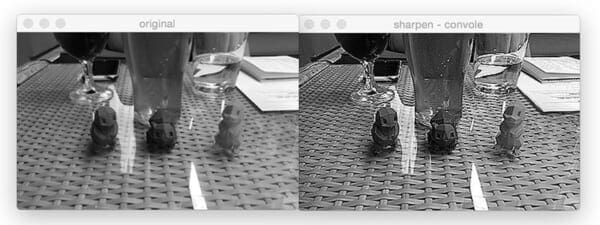
We define a sharpening kernel on Lines 58-61, used to enhance line structures and other details of an image. Explaining each of these kernels in detail is outside the scope of this tutorial, so if you’re interested in learning more about kernel construction, I would suggest starting here and then playing around with the excellent kernel visualization tool on Setosa.io.
Let’s define a few more kernels:
# construct the Laplacian kernel used to detect edge-like
# regions of an image
laplacian = np.array((
	[0, 1, 0],
	[1, -4, 1],
	[0, 1, 0]), dtype="int")

# construct the Sobel x-axis kernel
sobelX = np.array((
	[-1, 0, 1],
	[-2, 0, 2],
	[-1, 0, 1]), dtype="int")

# construct the Sobel y-axis kernel
sobelY = np.array((
	[-1, -2, -1],
	[0, 0, 0],
	[1, 2, 1]), dtype="int")
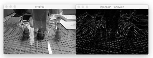
Lines 65-68 define a Laplacian operator that can be used as a form of edge detection.
Note: The Laplacian is also very useful for detecting blur in images.
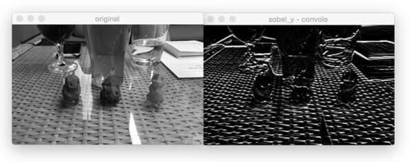
Finally, we’ll define two Sobel filters on Lines 71-80. The first (Lines 71-74) is used to detect vertical changes in the gradient of the image. Similarly, Lines 77-80 constructs a filter used to detect horizontal changes in the gradient.
Given all these kernels, we lump them together into a set of tuples called a “kernel bank”:
# construct the kernel bank, a list of kernels we're going
# to apply using both our custom `convole` function and
# OpenCV's `filter2D` function
kernelBank = (
	("small_blur", smallBlur),
	("large_blur", largeBlur),
	("sharpen", sharpen),
	("laplacian", laplacian),
	("sobel_x", sobelX),
	("sobel_y", sobelY)
)
Finally, we are ready to apply our kernelBank to our --input image:
# load the input image and convert it to grayscale
image = cv2.imread(args["image"])
gray = cv2.cvtColor(image, cv2.COLOR_BGR2GRAY)

# loop over the kernels
for (kernelName, kernel) in kernelBank:
	# apply the kernel to the grayscale image using both
	# our custom `convole` function and OpenCV's `filter2D`
	# function
	print("[INFO] applying {} kernel".format(kernelName))
	convoleOutput = convolve(gray, kernel)
	opencvOutput = cv2.filter2D(gray, -1, kernel)

	# show the output images
	cv2.imshow("original", gray)
	cv2.imshow("{} - convole".format(kernelName), convoleOutput)
	cv2.imshow("{} - opencv".format(kernelName), opencvOutput)
	cv2.waitKey(0)
	cv2.destroyAllWindows()
Lines 95 and 96 load our image from disk and convert it to grayscale. Convolution operators can certainly be applied to RGB (or other multi-channel images), but for the sake of simplicity in this blog post, we’ll only apply our filters to grayscale images).
We start looping over our set of kernels in the kernelBank on Line 99 and then apply the current kernel to the gray image on Line 104 by calling our custom convolve method which we defined earlier.
As a sanity check, we also call cv2.filter2D which also applies our kernel to the gray image. The cv2.filter2D function is a much more optimized version of our convolve function. The main reason I included the implementation of convolve in this blog post is to give you a better understanding of how convolutions work under the hood.
Finally, Lines 108-112 display the output images to our screen.
Example Convolutions with OpenCV and Python
Today’s example image comes from a photo I took a few weeks ago at my favorite bar in South Norwalk, CT — Cask Republic. In this image you’ll see a glass of my favorite beer (Smuttynose Findest Kind IPA) along with three 3D-printed Pokemon from the (unfortunately, now closed) Industrial Chimp shop:
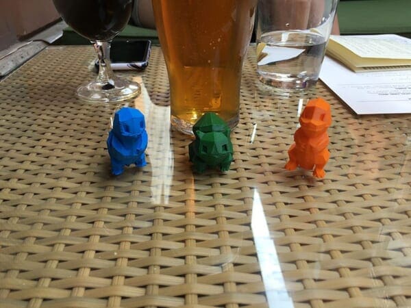
To run our script, just issue the following command:
$ python convolutions.py --image 3d_pokemon.png
You’ll then see the results of applying our smallBlur kernel to the input image:

On the left, we have our original image. Then in the center we have the results from the convolve function. And on the right, the results from cv2.filter2D . As the results demonstrate, our output matches cv2.filter2D , indicating that our convolve function is working properly. Furthermore, our original image now appears “blurred” and “smoothed”, thanks to the smoothing kernel.
Next, let’s apply a larger blur:
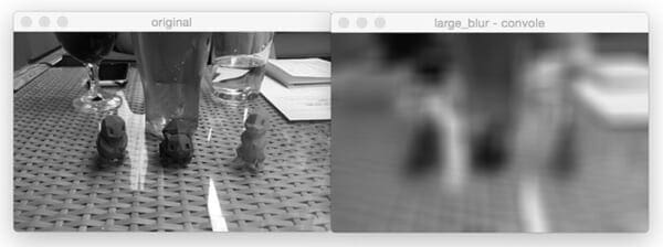
Comparing Figure 7 and Figure 8, notice how as the size of the averaging kernel increases, the amount of blur in the output image increases as well.
We can also sharpen our image:
Let’s compute edges using the Laplacian operator:
Find vertical edges with the Sobel operator:

And find horizontal edges using Sobel as well:
The Role of Convolutions in Deep Learning
As you’ve gathered through this blog post, we must manually hand-define each of our kernels for applying various operations such as smoothing, sharpening, and edge detection.
That’s all fine and good, but what if there was a way to learn these filters instead? Is it possible to define a machine learning algorithm that can look at images and eventually learn these types of operators?
In fact, there is — these types of algorithms are a sub-type of Neural Networks called Convolutional Neural Networks (CNNs). By applying convolutional filters, nonlinear activation functions, pooling, and backpropagation, CNNs are able to learn filters that can detect edges and blob-like structures in lower-level layers of the network — and then use the edges and structures as building blocks, eventually detecting higher-level objects (i.e., faces, cats, dogs, cups, etc.) in the deeper layers of the network.
Exactly how do CNNs do this?
I’ll show you — but it will have to wait for another few blog posts until we cover enough basics.
What's next? We recommend PyImageSearch University.
86+ total classes • 115+ hours hours of on-demand code walkthrough videos • Last updated: April 2026
★★★★★ 4.84 (128 Ratings) • 16,000+ Students Enrolled
I strongly believe that if you had the right teacher you could master computer vision and deep learning.
Do you think learning computer vision and deep learning has to be time-consuming, overwhelming, and complicated? Or has to involve complex mathematics and equations? Or requires a degree in computer science?
That’s not the case.
All you need to master computer vision and deep learning is for someone to explain things to you in simple, intuitive terms. And that’s exactly what I do. My mission is to change education and how complex Artificial Intelligence topics are taught.
If you're serious about learning computer vision, your next stop should be PyImageSearch University, the most comprehensive computer vision, deep learning, and OpenCV course online today. Here you’ll learn how to successfully and confidently apply computer vision to your work, research, and projects. Join me in computer vision mastery.
Inside PyImageSearch University you'll find:
- ✓ 86+ courses on essential computer vision, deep learning, and OpenCV topics
- ✓ 86 Certificates of Completion
- ✓ 115+ hours hours of on-demand video
- ✓ Brand new courses released regularly, ensuring you can keep up with state-of-the-art techniques
- ✓ Pre-configured Jupyter Notebooks in Google Colab
- ✓ Run all code examples in your web browser — works on Windows, macOS, and Linux (no dev environment configuration required!)
- ✓ Access to centralized code repos for all 540+ tutorials on PyImageSearch
- ✓ Easy one-click downloads for code, datasets, pre-trained models, etc.
- ✓ Access on mobile, laptop, desktop, etc.
Summary
In today’s blog post, we discussed image kernels and convolutions. If we think of an image as a big matrix, then an image kernel is just a tiny matrix that sits on top of the image.
This kernel then slides from left-to-right and top-to-bottom, computing the sum of element-wise multiplications between the input image and the kernel along the way — we call this value the kernel output. The kernel output is then stored in an output image at the same (x, y)-coordinates as the input image (after accounting for any padding to ensure the output image has the same dimensions as the input).
Given our newfound knowledge of convolutions, we defined an OpenCV and Python function to apply a series of kernels to an image. These operators allowed us to blur an image, sharpen it, and detect edges.
Finally, we briefly discussed the roles kernels/convolutions play in deep learning, specifically Convolutional Neural Networks, and how these filters can be learned automatically instead of needing to manually define them first.
In next week’s blog post, I’ll be showing you how to train your first Convolutional Neural Network from scratch using Python — be sure to signup for the PyImageSearch Newsletter using the form below to be notified when the blog post goes live!

Download the Source Code and FREE 17-page Resource Guide
Enter your email address below to get a .zip of the code and a FREE 17-page Resource Guide on Computer Vision, OpenCV, and Deep Learning. Inside you'll find my hand-picked tutorials, books, courses, and libraries to help you master CV and DL!

