How to plot accuracy and loss with mxnet

When it comes to high-performance deep learning on multiple GPUs (and not to mention, multiple machines) I tend to use the mxnet library.

Part of the Apache Incubator, mxnet is a flexible, efficient, and scalable library for deep learning (Amazon even uses it in their own in-house deep learning).

Inside the ImageNet Bundle of my book, Deep Learning for Computer Vision with Python, we use the mxnet library to reproduce the results of state-of-the-art publications and train deep neural networks on the massive ImageNet dataset, the de facto image classification benchmark (which consists of ~1.2 million images).

As scalable as mxnet is, unfortunately it misses some of the convenience functions we may find in Keras, TensorFlow/TensorBoard, and other deep learning libraries.

One of these convenience methods mxnet misses is plotting accuracy and loss over time.

The mxnet library logs training progress to your terminal or to file, similar to Caffe.

But in order to construct a plot displaying the accuracy and loss over time, we need to manually parse the logs.

In the future, I hope we can use the callback methods supplied by mxnet to obtain this information, but I’ve personally found them hard to use (especially when utilizing multiple GPUs or multiple machines).

Instead, I recommend that you parse the raw log files when building accuracy and loss plots with mxnet.

In today’s blog post I’ll demonstrate how you can parse a training log file from mxnet and then plot accuracy and loss over time — to learn how, just keep reading.

How to plot accuracy and loss with mxnet

In today’s tutorial, we’ll be plotting accuracy and loss using the mxnet library. The log file format changed slightly between mxnet v.0.11 and v0.12 so we’ll be covering both versions here.

In particular, we’ll be plotting:

• Training loss
• Validation loss
• Training rank-1 accuracy
• Validation rank-1 accuracy
• Training rank-5 accuracy
• Validation rank-5 accuracy

These six metrics are typically measured when training deep neural networks on the ImageNet dataset.

The associated log files we’ll be parsing come from our chapter on AlexNet inside Deep Learning for Computer Vision with Python where we train the seminal AlexNet architecture on the ImageNet dataset.

Interested in a free sample chapter of my book? The free Table of Contents + Sample Chapters includes ImageNet Bundle Chapter 5 “Training AlexNet on ImageNet”. Grab the free chapters by entering your email in the form at the bottom-right of this page.

When parsing mxnet log files we typically have one or more .log files residing on disk, like so:

(dl4cv) pyimagesearch@pyimagesearch-dl4cv:~/plot_log$ ls -al
total 108
drwxr-xr-x  2 pyimagesearch pyimagesearch  4096 Dec 25 15:46 .
drwxr-xr-x 23 pyimagesearch pyimagesearch  4096 Dec 25 16:48 ..
-rw-r--r--  1 pyimagesearch pyimagesearch  3974 Dec 25  2017 plot_log.py
-rw-r--r--  1 pyimagesearch pyimagesearch 60609 Dec 25  2017 training_0.log
-rw-r--r--  1 pyimagesearch pyimagesearch 20303 Dec 25  2017 training_65.log
-rw-r--r--  1 pyimagesearch pyimagesearch 12725 Dec 25  2017 training_85.log

Here you can see that I have three mxnet log files:

• training_0.log
• training_65.log
• training_85.log

The integer value in each of the log files is the starting epoch of when I started training my deep neural network.

When training a deep Convolutional Neural Network on a large dataset we typically have to:

1. Stop training
2. Reduce learning rate
3. Resume training from an earlier epoch

This process enables us to break out of local optima, descend into areas of lower loss, and increase our classification accuracy.

Based on the integer values in the file names above, you can see that I:

1. Started training from epoch zero (the first log file)
2. Stopped training, lowered the learning rate, and resumed training from epoch 65 (the second log file)
3. Stopped training again, this time at epoch 85, lowered the learning rate, and resumed training (the third and final log file)

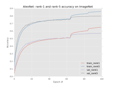
Our goal is to write a Python script that can parse the mxnet log files and create a plot similar to the one below that includes information on our training accuracy:

To get started, let’s take a look at an example of the mxnet training log format for mxnet <= 0.11 :

INFO:root:Epoch[73] Batch [500]	Speed: 1694.57 samples/sec	Train-accuracy=0.584035
INFO:root:Epoch[73] Batch [500]	Speed: 1694.57 samples/sec	Train-top_k_accuracy_5=0.816547
INFO:root:Epoch[73] Batch [500]	Speed: 1694.57 samples/sec	Train-cross-entropy=1.740517
INFO:root:Epoch[73] Batch [1000]	Speed: 1688.18 samples/sec	Train-accuracy=0.589742
INFO:root:Epoch[73] Batch [1000]	Speed: 1688.18 samples/sec	Train-top_k_accuracy_5=0.820633
INFO:root:Epoch[73] Batch [1000]	Speed: 1688.18 samples/sec	Train-cross-entropy=1.714734
INFO:root:Epoch[73] Resetting Data Iterator
INFO:root:Epoch[73] Time cost=728.322
INFO:root:Saved checkpoint to "imagenet/checkpoints/alexnet-0074.params"
INFO:root:Epoch[73] Validation-accuracy=0.559794
INFO:root:Epoch[73] Validation-top_k_accuracy_5=0.790751
INFO:root:Epoch[73] Validation-cross-entropy=1.914535

We can clearly see the epoch number inside the Epoch[*] text — this will make it easy to extract the epoch number.

All validation information, including validation accuracy, validation top-k (i.e., rank-5), and validation cross-entropy can be extracted by parsing out the following values:

• Validation-accuracy
• Validation-top_k_accuracy_5
• Validation-cross-entropy

The only tricky extraction is our training set information.

It would be nice if mxnet logged the final training accuracy and loss at the end of the epoch like they do for validation — but unfortunately, mxnet does not do this.

Instead, the mxnet library logs training information based on “batches”. After every N batches (where N is a user-supplied value during training), mxnet logs the training accuracy and loss to disk.

Therefore, if we extract the final batch values for:

• Train-accuracy
• Train-top_k_accuracy
• Train-cross-entropy

…we will be able to obtain an approximation to the training accuracy and loss for the given epoch.

You can make your training accuracy and loss more fine-grained or less verbose by adjusting the Speedometer callback during training.

Let’s move on to creating the plot_log.py file responsible for actually parsing the logs.

Open up a new file, name it plot_log.py , and insert the following code:

# import the necessary packages
import matplotlib.pyplot as plt
import numpy as np
import argparse
import re

# construct the argument parse and parse the arguments
ap = argparse.ArgumentParser()
ap.add_argument("-n", "--network", required=True,
	help="name of network")
ap.add_argument("-d", "--dataset", required=True,
	help="name of dataset")
args = vars(ap.parse_args())

Today we’ll also be making use of re , Python’s regular expression parser (Line 5).

I’ve always thought that Google’s documentation on the subject of regular expressions with Python is the best — be sure to check it out if you aren’t familiar with regular expression parsing in Python.

Another one of my favorite websites is Regex101.com. This site will allow you to test your regular expressions in the most popular coding languages. I’ve found it to be very helpful for development of parsing software.

Now that we’re armed with the tools needed to get today’s job done, let’s parse our command line arguments on Lines 8-13.

Our plot_log.py script requires two command line arguments:

• --network : The name of the network.
• --dataset : The name of the dataset.

We’ll reference these args later in the script.

Now we’re going to create a logs list:

# define the paths to the training logs
logs = [
	(65, "training_0.log"),			# lr=1e-2
	(85, "training_65.log"),		# lr=1e-3
	(100, "training_85.log"),		# lr=1e-4
]

Given that the logs list is a bit too tricky to include as command line arguments, I’ve hardcoded it here for this example script. You will need to edit this list when you plot your own logs.

An alternative would be to create a JSON (or equivalent) configuration file for each experiment and then load it from disk when you execute plot_logs.py .

As you can see on Lines 16-20, I’ve defined the log file paths along with the epochs they correspond to in a list of tuples.

Be sure to read the discussion above about the log file names above. In short, the filename itself contains the starting epoch and the first element of the tuple contains the ending epoch.

For this example, we have three log files as training was stopped twice to adjust the learning rate. You can easily add-to or remove-from this list as needed for your purposes.

From here we’ll just perform some compact list initializations:

# initialize the list of train rank-1 and rank-5 accuracies, along
# with the training loss
(trainRank1, trainRank5, trainLoss) = ([], [], [])

# initialize the list of validation rank-1 and rank-5 accuracies,
# along with the validation loss
(valRank1, valRank5, valLoss) = ([], [], [])

Lines 24 and 28 simply initialize variables to empty lists in a Pythonic way. We’ll be updating these lists shortly.

Now let’s loop over the logs and begin our regular expression matching:

# loop over the training logs
for (i, (endEpoch, p)) in enumerate(logs):
	# load the contents of the log file, then initialize the batch
	# lists for the training and validation data
	rows = open(p).read().strip()
	(bTrainRank1, bTrainRank5, bTrainLoss) = ([], [], [])
	(bValRank1, bValRank5, bValLoss) = ([], [], [])

	# grab the set of training epochs
	epochs = set(re.findall(r'Epoch\[(\d+)\]', rows))
	epochs = sorted([int(e) for e in epochs])

On Line 31 we begin our loop over logs , our list of tuples.

We open and read a log file on Line 34 while stripping unnecessary whitespace.

Training and validation data will be stored in batch lists, so we go ahead an initialize/set those lists to empty (Lines 35 and 36).

Caution: If you didn’t notice, let me point it out here that we have initialized 13 lists. It’s easy become confused regarding the purpose of each list. Thirteen also tends to be an unlucky number, so let’s clear things up right now. To clarify, the 6 lists beginning with a b are the batch lists — we’ll populate these in batches and then append element-wise (extend) them to the corresponding 6 training and validation lists which were defined before the loop. The 13th list, logs , is the easy one since it’s just our epoch numbers and log file paths. If you’re new to parsing logs or having trouble following the code make sure you insert print statements to debug and ensure you’re understanding what the code is doing.

Our first use of re is on Line 39. Here we are parsing the epoch numbers from the rows in the log files.

As we know from earlier in this post, the log files contain Epoch[*] , so if you read carefully you’ll see we’re extracting the decimal digits, \d+ , from within the brackets. Be sure to refer to the Google Python Regular Expression documentation to understand the syntax, or read ahead where I’ll explain the next regular expression in more detail.

Sorting the epochs found by this regular expression is taken care of on Line 40.

Now we’re going to loop over each epoch in the list and extract + append training information to the corresponding lists:

	# loop over the epochs
	for e in epochs:
		# find all rank-1 accuracies, rank-5 accuracies, and loss
		# values, then take the final entry in the list for each
		s = r'Epoch\[' + str(e) + '\].*Train-accuracy=(.*)'
		rank1 = re.findall(s, rows)[-1]
		s = r'Epoch\[' + str(e) + '\].*Train-top_k_accuracy_5=(.*)'
		rank5 = re.findall(s, rows)[-1]
		s = r'Epoch\[' + str(e) + '\].*Train-cross-entropy=(.*)'
		loss = re.findall(s, rows)[-1]

		# update the batch training lists
		bTrainRank1.append(float(rank1))
		bTrainRank5.append(float(rank5))
		bTrainLoss.append(float(loss))

On Line 43 we begin to loop over all the epochs.

We are extracting three values:

• Train-accuracy : Our rank-1 accuracy.
• Train-top_k_accuracy_5 : This is our rank-5 accuracy.
• Train-cross-entropy : This value is our loss.

…and to do this cleanly, each extraction spans two lines of code.

I’ll break down the rank-1 accuracy extraction on Lines 46 and 47 — the other extractions follow the same format.

For epoch 3, batch 500, the log file looks like so (beginning on Line 38):

INFO:root:Epoch[3] Batch [500]	Speed: 1692.63 samples/sec	Train-accuracy=0.159705
INFO:root:Epoch[3] Batch [500]	Speed: 1692.63 samples/sec	Train-top_k_accuracy_5=0.352742
INFO:root:Epoch[3] Batch [500]	Speed: 1692.63 samples/sec	Train-cross-entropy=4.523639

The rank-1 accuracy is at the end of Line 38 after the “=”.

So we’re looking for “Epoch[3]” + <any char(s)> + “Train-accuracy=” + <the rank-1 float value>.

First, we build our regex format string, s . What we’re matching (looking for) is mostly spelled out, however there are some special regex formatting characters mixed in:

• The backslashes (‘\’) are escape characters. Because we’re explicitly looking for ‘[‘ and ‘]’ we place a backslash before each.
• The “.*” means any character(s) — in this case it is in the middle of the format string which implies that there there could be any character(s) in-between.
• The key characters are the ‘(‘ and ‘)’, which mark our extraction. In this case, we’re extracting the characters right after the ‘=’ in the row.

Then, after we’ve constructed s , on the subsequent line we call re.findall . Using our format string, s , and rows , the re.findall function finds all matches and extracts the rank-1 accuracies. Magic!

Sidenote: We’re only interested in the last value, hence the [-1] list index.

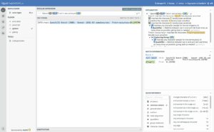
To see this Python regular expression in action, let’s look at a screenshot from Regex101.com (click image to enlarge):

Again, I highly recommend Regex101 to get started with regular expressions. It is also quite useful for parsing advanced and complex strings (luckily ours are relatively easy).

The next two expressions are parsed in the same way on Lines 48-51.

We’ve successfully extracted the values, so the next step is to append the values to their respective lists in floating point form on Lines 54-56.

From there, we can grab the validation information in the same way:

	# extract the validation rank-1 and rank-5 accuracies for each
	# epoch, followed by the loss
	bValRank1 = re.findall(r'Validation-accuracy=(.*)', rows)
	bValRank5 = re.findall(r'Validation-top_k_accuracy_5=(.*)', rows)
	bValLoss = re.findall(r'Validation-cross-entropy=(.*)', rows)

	# convert the validation rank-1, rank-5, and loss lists to floats
	bValRank1 = [float(x) for x in bValRank1]
	bValRank5 = [float(x) for x in bValRank5]
	bValLoss = [float(x) for x in bValLoss]

I won’t go through the intricacies of a regular expression match again. So be sure to study the above example and apply it to Lines 60-63 where we extract the validation rank-1, rank-5, and loss values. If you need to, plug in log file data and the regular expression string into Regex101, as shown in Figure 2.

As before, we convert the strings to floats (with list-comprehension here) and append the lists to the respective batch lists (Lines 65-67).

Next, we’ll figure out our array slices so that we can update the lists we’ll use for plotting:

	# check to see if we are examining a log file other than the
	# first one, and if so, use the number of the final epoch in
	# the log file as our slice index
	if i > 0 and endEpoch is not None:
		trainEnd = endEpoch - logs[i - 1][0]
		valEnd = endEpoch - logs[i - 1][0]

	# otherwise, this is the first epoch so no subtraction needs
	# to be done
	else:
		trainEnd = endEpoch
		valEnd = endEpoch

Here, we need to set trainEnd and valEnd . These temporary values will be used for slicing.

To do so, we check which log file is currently being parsed. We know which log is being parsed as we enumerated the values when we started the loop.

If we happen to be examining a log other than the first one, we’ll use the epoch number of the final epoch in the log file as our slice index (Lines 72-74).

Otherwise, no subtraction needs to happen, so we simply set the trainEnd and valEnd to the endEpoch (Lines 78-80).

Last but certainly not least, we need to update the training and validation lists:

	# update the training lists
	trainRank1.extend(bTrainRank1[0:trainEnd])
	trainRank5.extend(bTrainRank5[0:trainEnd])
	trainLoss.extend(bTrainLoss[0:trainEnd])

	# update the validation lists
	valRank1.extend(bValRank1[0:valEnd])
	valRank5.extend(bValRank5[0:valEnd])
	valLoss.extend(bValLoss[0:valEnd])

Using the batch lists from each iteration of the loop, we append them element-wise (this is known as extending in Python) to the respective training (Lines 83-85) and validation lists (Lines 88-90).

After we iterate through each of the log files, we have 6 convenient lists ready to be plotted.

Now that our data is parsed and organized in those helpful lists, let’s go ahead and construct the plots with matplotlib:

# plot the accuracies
plt.style.use("ggplot")
plt.figure()
plt.plot(np.arange(0, len(trainRank1)), trainRank1,
	label="train_rank1")
plt.plot(np.arange(0, len(trainRank5)), trainRank5,
	label="train_rank5")
plt.plot(np.arange(0, len(valRank1)), valRank1,
	label="val_rank1")
plt.plot(np.arange(0, len(valRank5)), valRank5,
	label="val_rank5")
plt.title("{}: rank-1 and rank-5 accuracy on {}".format(
	args["network"], args["dataset"]))
plt.xlabel("Epoch #")
plt.ylabel("Accuracy")
plt.legend(loc="lower right")

Here we are plotting rank-1 and rank-5 accuracies for training + validation. We also give our plot a title from our command line args.

Similarly, let’s plot training + validation losses:

# plot the losses
plt.style.use("ggplot")
plt.figure()
plt.plot(np.arange(0, len(trainLoss)), trainLoss,
	label="train_loss")
plt.plot(np.arange(0, len(valLoss)), valLoss,
	label="val_loss")
plt.title("{}: cross-entropy loss on {}".format(args["network"],
	args["dataset"]))
plt.xlabel("Epoch #")
plt.ylabel("Loss")
plt.legend(loc="upper right")
plt.show()

In mxnet 0.12 and above, the format of the log file changed slightly.

The main difference is that training accuracy and loss are now displayed on the same line. Here’s an example from Epoch 3, batch 500 again:

INFO:root:Epoch[3] Batch [500]	Speed: 1997.40 samples/sec	accuracy=0.013391	top_k_accuracy_5=0.048828	cross-entropy=6.878449

Be sure to scroll right to see Line 47‘s full output.

Thanks to Dr. Daniel Bonner of ANU Medical School in Australia, we have an updated script:

	# loop over the epochs
	for e in epochs:
		# find all rank-1 accuracies, rank-5 accuracies, and loss
		# values, then take the final entry in the list for each
		s = r'Epoch\[' + str(e) + '\].*accuracy=([0]*\.?[0-9]+)'
		rank1 = re.findall(s, rows)[-2]
		s = r'Epoch\[' + str(e) + '\].*top_k_accuracy_5=([0]*\.?[0-9]+)'
		rank5 = re.findall(s, rows)[-2]
		s = r'Epoch\[' + str(e) + '\].*cross-entropy=([0-9]*\.?[0-9]+)'
		loss = re.findall(s, rows)[-2]

		# update the batch training lists
		bTrainRank1.append(float(rank1))
		bTrainRank5.append(float(rank5))
		bTrainLoss.append(float(loss))

Be sure to see the “Downloads” section below where you can download both versions of the script.

Results

I trained Krizhevsky et al.’s AlexNet CNN on the ImageNet dataset using the mxnet framework, as is detailed in my book, Deep Learning for Computer Vision with Python.

Along the way, I stopped/started the training process while adjusting the learning rate. This process produced the three log files aforementioned.

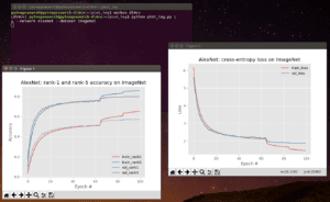
Now with one command, using the method described in this blog post, I have parsed all three log files and generated training progress plots with matplotlib:

$ python plot_log.py --network AlexNet --dataset ImageNet

Summary

In today’s blog post we learned how to parse mxnet log files, extract training and validation information (including loss and accuracy), and then plot this information over time.

Parsing mxnet logs can be a bit tedious so I hope the code provided in this blog post helps you out.

If you’re interested in learning how to train your own Convolutional Neural Networks using the mxnet library, be sure to take a look at the ImageNet Bundle of my new book, Deep Learning for Computer Vision with Python.

Otherwise, be sure to enter your email address in the form below to be notified when future blog posts go live!