Credit Card Fraud Detection Using Spectral Clustering

---

Table of Contents

---

Credit Card Fraud Detection Using Spectral Clustering

In this tutorial, you will learn how to use Spectral Clustering for credit card fraud detection.

In today’s digital age, credit card fraud (Figure 1) has become a significant concern for both consumers and financial institutions. With the increasing volume of online transactions, the need for robust and efficient fraud detection systems is more critical than ever. Traditional methods often fall short in identifying sophisticated fraudulent activities, making it essential to explore advanced techniques.

One such promising approach is anomaly detection, which focuses on identifying unusual patterns that deviate from the norm. By leveraging anomaly detection, we can uncover hidden irregularities in transaction data that may indicate fraudulent behavior.

Spectral clustering, a technique rooted in graph theory, offers a unique way to detect anomalies by transforming data into a graph and analyzing its spectral properties. This method excels in identifying clusters of similar transactions and isolating those that deviate from the norm.

In this tutorial, we will delve into the fundamentals of anomaly detection and understand how spectral clustering can be used for credit card fraud detection.

This lesson is the 1st of a 4-part series on Anomaly Detection 101:

1. Credit Card Fraud Detection Using Spectral Clustering (this tutorial)
2. Predictive Maintenance Using Isolation Forest
3. Build a Network Intrusion Detection System with Variational Autoencoders
4. Outlier Detection Using the Grubbs Test

To learn how to use Spectral Clustering for credit card fraud detection, just keep reading.

---

Understanding Anomaly Detection: Concepts, Types, and Algorithms

---

What Is Anomaly Detection?

Anomaly detection (Figure 2) is a critical technique in data analysis used to identify data points, events, or observations that deviate significantly from the norm. These deviations, known as anomalies or outliers, can indicate important and often actionable insights (e.g., fraud, network intrusions, or system failures).

The primary objective of anomaly detection is to distinguish between normal and abnormal patterns within a dataset, enabling timely intervention and mitigation of potential risks.

---

Applications of Anomaly Detection

Figure 3 explains several applications of anomaly detection in various areas. For example,

• Credit Card Fraud Detection: In the context of credit card transactions, anomaly detection can be used to identify fraudulent activities. For example, if a credit card is suddenly used to make a large purchase in a foreign country, this transaction might be flagged as an anomaly. By analyzing the patterns of normal transactions, the system can detect unusual activities that deviate from the norm.
• Network Intrusion Detection: In cybersecurity, anomaly detection is used to identify potential network intrusions. For instance, if a user who typically accesses the network during business hours suddenly logs in at midnight and starts downloading large amounts of data, this behavior would be considered anomalous. The system can then alert administrators to investigate further.
• Industrial Equipment Monitoring or Predictive Maintenance: In industrial settings, anomaly detection can be used to monitor equipment for potential failures. For example, if a machine that usually operates within a specific temperature range suddenly shows a spike in temperature, this could indicate a malfunction. Early detection of such anomalies can prevent costly downtime and repairs.

---

Types of Anomaly Detection Problems

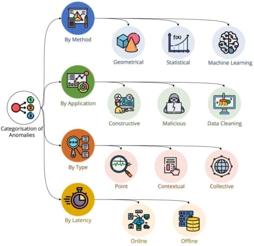
Anomaly detection problems can be broadly categorized into three main types:

• point anomalies
• contextual anomalies
• collective anomalies

Each type (Figure 4) has distinct characteristics and applications, making it essential to understand their differences and how they can be effectively identified.

---

Point Anomalies

Point anomalies, also known as global anomalies, occur when an individual data point significantly deviates from the rest of the data. These anomalies are the simplest to detect because they stand out clearly against the background of normal data.

For example, a single transaction that is much larger than usual or occurs in an unusual location can be flagged as a point anomaly.

---

Contextual Anomalies

Contextual anomalies, also known as conditional anomalies, occur when a data point is considered anomalous in a specific context but may be normal in another. The context is defined by the surrounding data points or additional contextual attributes.

For example, a high-temperature reading might be normal during the day but anomalous at night. The context here is the time of day.

---

Collective Anomalies

Collective anomalies occur when a collection of related data points is anomalous, even if individual points within the collection are not. These anomalies are identified based on the relationship between data points rather than their values.

For example, a series of small data packets sent in a short period might be normal individually, but collectively, they could indicate a denial-of-service (DoS) attack.

---

Algorithms for Anomaly Detection

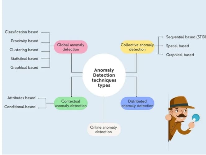
We can divide anomaly detection algorithms (Figure 5) into the following:

• statistical methods
• machine learning methods
• proximity-based methods
• ensemble methods

---

Statistical Methods

Statistical methods rely on the assumption that normal data points follow a specific statistical distribution. Anomalies are identified as data points that deviate significantly from this distribution.

For example, the Z-Score method (Figure 6) calculates the Z-score for each data point, which measures how many standard deviations a point is from the mean. Data points with a Z-score above a certain threshold are considered anomalies.

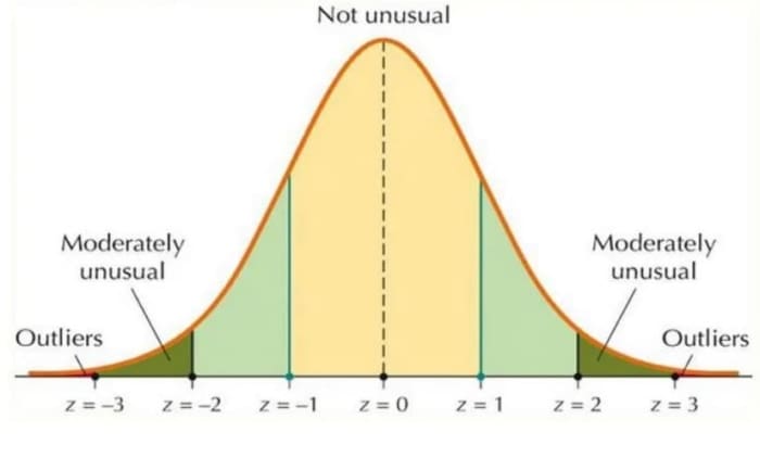
Such a method can be applicable in scenarios (e.g., credit card transactions), where a transaction with a Z-score of 5 might be flagged as an anomaly because it is far from the average transaction amount.

---

Machine Learning Methods

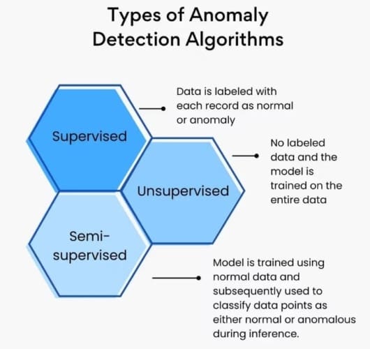
Machine learning methods (Figure 7) can be divided into supervised, unsupervised, and semi-supervised learning techniques.

Supervised Learning

These methods require labeled data to train the model. The model learns to distinguish between normal and abnormal data points.

For example, in fraud detection, SVM (support vector machine) can classify transactions as fraudulent or non-fraudulent based on historically labeled data.

Similarly, neural network techniques like Convolutional Neural Networks (CNNs) and Recurrent Neural Networks (RNNs) can be used for image and time-series data to detect defects in products by learning from labeled images of defective and non-defective products.

Unsupervised Learning

These methods do not require labeled data and can identify anomalies based on the inherent structure of the data.

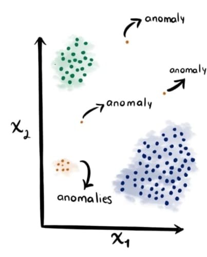
For example, clustering algorithms (e.g., K-Means, Spectral Clustering, and DBSCAN (Density-Based Spatial Clustering of Applications with Noise)) are used to partition data into clusters. Data points that do not belong to any cluster or are far from the cluster centroids are considered anomalies.

For instance, in customer segmentation, K-means clustering can identify customers whose purchasing behavior is significantly different from the majority.

Semi-Supervised Learning

These methods use a small amount of labeled data to guide the learning process.

For example, in network security, One-Class SVM can be trained only on normal traffic data and used to identify point anomalies (e.g., unusual network traffic patterns).

Similarly, autoencoders can be trained to reconstruct input data, and data points with high reconstruction errors can be flagged as anomalies.

---

Proximity-Based Methods

Proximity-based methods can detect anomalies based on the distance between data points. For example, The K-Nearest Neighbors algorithm can identify unusual login attempts based on the distance to typical login patterns.

The Local Outlier Factor (LOF) algorithm measures the local density deviation of a data point with respect to its neighbors. Points with a significantly lower density than their neighbors are considered anomalies.

---

Ensemble Methods

Ensemble methods combine multiple algorithms to improve the accuracy and robustness of anomaly detection. For example,

The Isolation Forest algorithm (Figure 8) isolates anomalies by randomly selecting a feature and splitting the data. Because of this, anomalies are isolated quickly because they are rare and different.

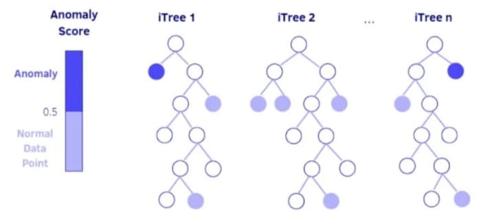
Similar to the Isolation Forest, the Random-Cut Forest uses random cuts to partition the data. Anomalies are identified based on the number of cuts required to isolate them.

---

Understanding Spectral Clustering

---

Basics of Clustering Techniques: K-Means Algorithm

Clustering is a fundamental technique in unsupervised machine learning used to group similar data points. Unlike supervised learning, where the model is trained on labeled data, clustering algorithms work on unlabeled data, identifying inherent structures within the data. This technique is widely used in various fields (e.g., market research, image segmentation, and bioinformatics).

Figure 9 displays how clustering can help in anomaly detection.

---

K-Means Clustering

K-Means (Figure 10) is one of the most popular clustering algorithms due to its simplicity and efficiency. The goal of K-Means is to partition a dataset into K distinct, non-overlapping subsets (clusters). Each data point belongs to the cluster with the nearest mean, serving as a prototype of the cluster.

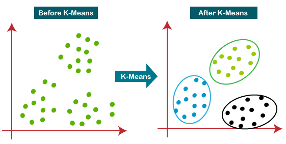
The K-Means algorithm follows these steps:

Initialization

• Randomly select data points as initial centroids.
• These centroids can be chosen randomly or use methods like K-Means++ to improve convergence.

Assignment

• For each data point, calculate the distance to each centroid.
• Assign the data point to the cluster with the nearest centroid.

Update

• Recalculate the centroid of each cluster by taking the mean of all data points in the cluster.
• The new centroid is the average position of all the points in the cluster.

Convergence

• Repeat the assignment and update steps until the centroids do not change significantly.
• Alternatively, stop after a predefined number of iterations.

---

Choosing the Number of Clusters (K)

Selecting the right number of clusters is crucial for the effectiveness of K-Means.

The Elbow Method (Figure 11) is a heuristic used in determining the optimal number of clusters in K-Means clustering. The method involves running the K-Means algorithm on the dataset for a range of values of (number of clusters), and for each value of , calculating the sum of squared distances from each point to its assigned cluster centroid, known as the Within-Cluster Sum of Squares (WCSS).

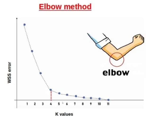
These WCSS values are then plotted against the number of clusters. As the number of clusters increases, the WCSS typically decreases because the points are closer to their centroids. However, there is a point where the rate of decrease sharply slows down, forming an “elbow” shape in the plot. This point, known as the “elbow point,” suggests the optimal number of clusters, as adding more clusters beyond this point yields diminishing returns in terms of reducing WCSS.

---

Introduction to Spectral Clustering

---

Disadvantages of K-Means

• Assumption of Spherical Clusters: K-Means assumes that clusters are spherical and evenly sized, which is not always the case in real-world data.
• Sensitivity to Initial Centroids: The algorithm’s performance heavily depends on the initial placement of centroids, which can lead to suboptimal clustering.
• Difficulty with Non-Linearly Separable Data: K-Means struggles with data that is not linearly separable, as it relies on Euclidean distance.
• Fixed Number of Clusters: The number of clusters (K) must be specified in advance, which is not always straightforward.

---

How Spectral Clustering Works

Spectral clustering (Figure 12) overcomes many of the limitations of K-Means by considering the data points as nodes of a graph and edge weights as a measure of similarity between two nodes.

The eigenvalues (spectrum) of a similarity matrix are used to reduce the dimensions of the data points before clustering, which allows spectral clustering to exploit the intrinsic structure of the data and handle non-linearly separable data and clusters of arbitrary shapes more effectively.

Spectral clustering is particularly effective for anomaly detection because it can handle complex, non-linear data structures and identify clusters that traditional methods might miss.

Spectral clustering involves the following steps:

Constructing the Similarity Matrix:

• Given data points (), we represent them as nodes in a graph.
• The similarity matrix stores the similarity of each node pair. It can be constructed using various methods, such as Gaussian similarity:

• where is a scaling parameter. The closer the two nodes and are, the more similar they will be.

Computing the Laplacian Matrix:

• The degree matrix is calculated as:

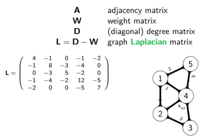
• The unnormalized Laplacian matrix (Figure 13) is then:

Computing Eigenvalues and Eigenvectors:

• Solve the eigenvalue problem for :

• where are the eigenvalues and are the eigenvectors.
• Select the eigenvectors corresponding to the smallest eigenvalues to form the matrix .

Clustering the Data:

• Apply K-Means to the rows of to obtain the final clusters.

---

Choosing the Number of Clusters (K)

The Eigengap Heuristic (Figure 14) is a method used in spectral clustering to determine the optimal number of clusters by examining the eigenvalues of the graph Laplacian matrix.

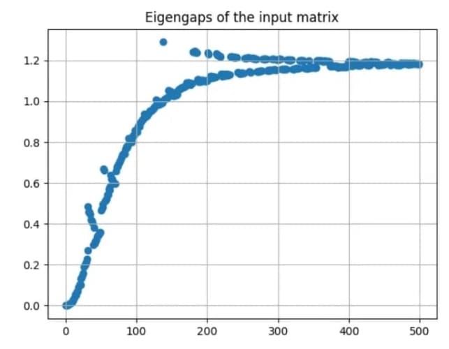
The idea is to plot the eigenvalues of graph Laplacian in ascending order. The optimal number of clusters, , is typically chosen where there is a significant gap between consecutive eigenvalues. This large gap indicates a clear separation between clusters. Mathematically, is chosen such that:

where and are two consecutive eigenvalues.

The rationale is that the eigenvalues reflect the “smoothness” of the data partitioning, and a large gap implies that adding more clusters beyond this point would not significantly improve the separation. Therefore, the optimal number of clusters, , is chosen where this largest gap is observed, leveraging the inherent structure of the data to guide the clustering process.

---

Spectral Clustering for Credit Card Fraud Detection

In this section, we will implement a project to use Spectral Clustering for credit card fraud detection. With the increasing volume of online transactions, credit card fraud has become a significant concern for both consumers and financial institutions. Hence, we need robust and reliable fraud detection systems.

We will start by setting up libraries and data preparation.

---

Setup and Data Preparation

To start, we will first download the Credit Card Fraud Detection dataset, which contains details (e.g., transaction amount, transaction date, total card declines in a day, average transaction per day, etc.) for 3000+ credit card transactions. Out of 3000 transactions, 450 transactions are marked fraudulent. Our goal is to identify these fraudulent transactions using Anomaly detection correctly.

To download our dataset and set up our environment, we will install the following packages.

• kaggle: command line API for downloading the datasets from Kaggle
• pandas: to load our dataset files
• scipy: to use statistical measures like z-score
• matplotlib: to plot and visualize the dataset and clusters
• scikit-learn: for standard preprocessing and K-means clustering functions

$ pip install kaggle pandas matplotlib scikit-learn scipy
$ kaggle datasets download -d shubhamjoshi2130of/abstract-data-set-for-credit-card-fraud-detection
$ unzip /content/abstract-data-set-for-credit-card-fraud-detection.zip -d /content/

After downloading the dataset, we will now load our credit card transactions dataset, preprocess various features and then visualize them via Matplotlib plots.

import pandas as pd
import matplotlib.pyplot as plt

data = pd.read_csv("/content/creditcardcsvpresent.csv", header='infer')


data["Is declined"] = data["Is declined"].apply(lambda x: 1 if x=='Y' else 0)
data["isForeignTransaction"] = data["isForeignTransaction"].apply(lambda x: 1 if x=='Y' else 0)
data["isHighRiskCountry"] = data["isHighRiskCountry"].apply(lambda x: 1 if x=='Y' else 0)
data["isFradulent"] = data["isFradulent"].apply(lambda x: 1 if x=='Y' else 0)

data = data.drop(["Merchant_id","Transaction date"], axis=1)

print(data.head())
print(data.isFradulent.value_counts())

# Plotting the distribution of all columns
data.hist(bins=50, figsize=(20, 15))
plt.suptitle('Distribution of All Columns')
plt.show()

In the provided code, we start by importing the necessary libraries, pandas and matplotlib.pyplot (Lines 1 and 2). We then read a CSV file named creditcardcsvpresent.csv into a DataFrame using pd.read_csv() with the header inferred (Line 4).

Next, we convert specific columns to binary values: "Is declined", "isForeignTransaction", "isHighRiskCountry", and "isFradulent" are transformed such that 'Y' becomes 1 and any other value becomes 0 (Lines 7-10). This is done using the apply() function with a lambda function. We also drop the "Merchant_id" and "Transaction date" columns from the DataFrame as they don’t provide any meaningful information (Line 12).

After preprocessing the data, we print the first few rows of the DataFrame to verify the changes (Lines 14 and 15). Finally, we plot the distribution of all columns in the DataFrame using the hist() method (Lines 18 and 19). This helps us visualize the data distribution across different features.

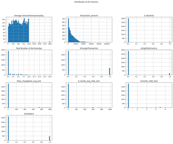
Figure 15 displays the distribution of different columns (features) of the dataset.

Next, we normalize our dataset features using the Sklearn MinMaxScaler.

The MinMaxScaler transforms features by scaling each feature to a given range, typically between 0 and 1. The formula used by the MinMaxScaler is:

Here, is the original value, is the minimum value of the feature, and is the maximum value of the feature. This transformation ensures that the scaled values fall within the specified range, preserving the relationships between the original data points while normalizing the scale.

from sklearn.preprocessing import MinMaxScaler
scaler = MinMaxScaler()

X = data.loc[:, data.columns != 'isFradulent'].to_numpy()
y_true = data["isFradulent"].to_numpy()

X_scaled = scaler.fit_transform(X)
print(X.shape)

In this code, we first import the MinMaxScaler and StandardScaler from the sklearn.preprocessing module (Line 21), and then create an instance of MinMaxScaler (Line 22).

We extract the feature matrix X by selecting all columns except 'isFradulent' and convert it to a NumPy array (Line 24). Similarly, we extract the target variable y_true from the 'isFradulent' column and convert it to a NumPy array (Line 25). We then scale the feature matrix X using the fit_transform method of the MinMaxScaler instance, storing the result in X_scaled (Line 27). Finally, we print the shape of the original feature matrix X to verify its dimensions (Line 28).

---

Implementing Spectral Clustering

Now that we have loaded, visualized, and pre-processed our dataset, it is time to implement the spectral clustering algorithm.

import numpy as np
from sklearn.cluster import KMeans
from sklearn.metrics import pairwise_kernels

def laplacian_eigen_decomposition(X, sigma=1.0):
    # Step 1: Construct the similarity matrix
    W = pairwise_kernels(X, metric='rbf', gamma=1/(2*sigma**2))

    # Step 2: Compute the degree matrix
    D = np.diag(np.sum(W, axis=1))

    # Step 3: Compute the graph Laplacian
    L_sym = D -  W

    # Step 4: Eigenvalue decomposition
    eigvals, eigvecs = np.linalg.eigh(L_sym)

    return eigvals, eigvecs

def clustering(U, k):
    # Step 5: Normalize rows of U
    U_normalized = U / np.linalg.norm(U, axis=1, keepdims=True)

    # Step 6: Apply k-means to rows of U
    kmeans = KMeans(n_clusters=k)
    labels = kmeans.fit_predict(U_normalized)

    return labels, kmeans.cluster_centers_

Here, we are implementing a spectral clustering algorithm, which involves using the eigenvalues and eigenvectors of a graph Laplacian matrix to perform clustering. We start by importing necessary libraries: numpy for numerical operations, KMeans from sklearn.cluster for clustering, and pairwise_kernels from sklearn.metrics for computing the similarity matrix (Lines 29-31).

The function laplacian_eigen_decomposition takes a dataset X and a parameter sigma to construct the similarity matrix W using the radial basis function (RBF) kernel (Lines 34 and 35). The degree matrix D is then computed as a diagonal matrix where each diagonal element is the sum of the corresponding row in W (Line 38).

We then compute the symmetric graph Laplacian L_sym by subtracting W from D (Line 41). Finally, we perform eigenvalue decomposition on L_sym to obtain its eigenvalues and eigenvectors, which are returned by the function (Lines 44-46).

The second function, clustering, takes the eigenvectors U and the number of clusters k as inputs. We start by normalizing the rows of U to ensure that each row has a unit norm (Line 50). This normalization step is crucial as it helps in stabilizing the clustering process.

We then apply the k-means algorithm to the normalized rows of U to assign each data point to one of the k clusters (Lines 53 and 54). The function returns the cluster labels and the cluster centers determined by k-means (Line 56). This approach leverages the spectral properties of the data to perform clustering, which can be particularly effective for identifying clusters in complex datasets.

Now, we will use these functions to partition our dataset into clusters. First, we will compute and plot the eigenvalues of the graph Laplacian in ascending order.

eigvals, eigvecs = laplacian_eigen_decomposition(X_scaled, sigma=1)
print(eigvals)

# plot of eigen values
plt.ylabel('EigenValues')
plt.xlabel('K-values')
plt.plot(np.array(eigvals).tolist(), linestyle='--', marker='o', color='b')
plt.show()

Figure 16 displays the eigenvalues of the graph Laplacian plotted in ascending order.

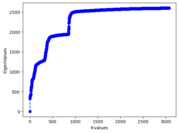
From the plot, we can see that there is a large gap between the first and second eigenvalues. The Eigengap heuristic indicates that we will ideally need only one cluster to identify fraudulent transactions. However, in this project, we will cluster the dataset into 2 partitions so that we can show the next steps involved in the spectral clustering. Ideally choosing one or two clusters in this case should result in similar performance.

K = 2
U = eigvecs[:, :K]
cluster_labels, cluster_centers = clustering(U, k=K)

# Plot the clusters
U_normalized = U / np.linalg.norm(U, axis=1, keepdims=True)
plt.scatter(U_normalized[:, 0], U_normalized[:, 1], c=cluster_labels, s=30)

# Plot the centroids
plt.scatter(cluster_centers[:, 0], cluster_centers[:, 1], c='red', s=200, alpha=0.75, marker='X')
plt.show()

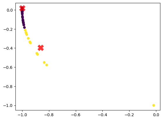
In the above code, we apply K-Means clustering to the first K rows of eigvecs (post normalization) to obtain the final cluster labels.

Figure 17 shows the clusters and cluster centroids.

---

Identifying Fraudulent Transactions

In the previous section, we clustered our dataset using spectral clustering. But how do we use these cluster assignments to identify point anomalies (or fraudulent transactions)?

The idea is to iterate through each cluster and flag those data points which deviate significantly from their corresponding distribution.

For measuring this deviation, we can use the Z-Score method that measures how many standard deviations a point is from the mean (cluster centroid in this case). Data points with a Z-score above a certain threshold (e.g., 2) are considered anomalies (or fraudulent transactions). The Z-score for a data point in cluster can be calculated using the following formula:

where represents the value of the data point, is the mean of the th cluster or cluster centroid, and is the standard deviation of the th cluster.

This formula helps us understand how far a particular data point is from the mean of its cluster, measured in terms of standard deviations. A positive Z-score indicates that the data point is above the mean, while a negative Z-score indicates it is below the mean.

The following code uses the Z-score to identify fraudulent transactions in each cluster.

from scipy.stats import zscore
from sklearn.metrics import precision_score, recall_score

z_score_threshold = 2
# Identify fraud transactions within each cluster using z-score method
fraud_predictions = pd.Series(0, index=data.index)  # Initialize all as non-fraud
for cluster in range(K):
    cluster_data = X_scaled[cluster_labels == cluster]
    print(f"Data points in cluster {cluster} : {cluster_data.shape[0]}")
    cluster_z_scores = zscore(cluster_data)
    fraud_indices = (abs(cluster_z_scores) > z_score_threshold).any(axis=1)  # Identify outliers
    fraud_predictions[cluster_labels == cluster] = fraud_indices.astype(np.int64)

fraud_predictions = fraud_predictions.to_numpy(dtype='int64')

We start by importing necessary functions and initializing a fraud_predictions Series with all values set to 0 (Lines 76-81). For each cluster, we extract the data points, calculate their Z-scores, and identify outliers with an absolute Z-score greater than z_score_threshold (currently set to 2) (Lines 81-86). These outliers are marked as fraudulent in the fraud_predictions Series (Lines 86 and 87).

Now that we have our predictions, we will evaluate them against the ground truth. In the context of credit card fraud detection, precision and recall are crucial metrics for evaluating the performance of a fraud detection model.

Precision measures the accuracy of the model’s positive predictions. It is defined as the ratio of correctly identified fraudulent transactions (true frauds) to the total number of transactions predicted as fraudulent (predicted frauds). The formula for precision is:

Recall, also known as sensitivity or true positive rate, measures the model’s ability to identify all actual fraudulent transactions. It is defined as the ratio of correctly identified fraudulent transactions (true frauds) to the total number of actual fraudulent transactions (true frauds plus missed frauds). The formula for recall is:

High recall ensures that most fraudulent transactions are detected, while high precision ensures that the detected frauds are mostly correct. Balancing these metrics is key to an effective fraud detection system.

The following code computes the precision and recall of our algorithm.

# Calculate precision and recall
precision = precision_score(y_true, fraud_predictions)
recall = recall_score(y_true, fraud_predictions)

print(f'Precision: {precision:.2f}')
print(f'Recall: {recall:.2f}')

Output:

Precision: 0.73
Recall: 0.88

From the output of the above code, our spectral clustering-based anomaly detection algorithm gives a precision of 73% and recall of 88%, which is considered quite good.

Further, we can trade off precision and recall by controlling the z_score_threshold, which is currently set to 2. Lowering the z_score_threshold will improve recall but lower precision, while increasing it will improve precision but lower recall.

---

---

Summary

In this tutorial, we delve into the fascinating world of anomaly detection, specifically focusing on credit card fraud detection using spectral clustering. We begin by exploring the fundamental concepts, types, and algorithms associated with anomaly detection. This includes understanding what anomaly detection is, its various applications, and the different types of anomaly detection problems (e.g., point anomalies, contextual anomalies, and collective anomalies). We also discuss the various algorithms used for anomaly detection (e.g., statistical methods, machine learning methods, proximity-based methods, and ensemble methods).

Next, we shift our focus to spectral clustering, a powerful technique for identifying patterns in data. We start with the basics of clustering techniques, particularly the K-Means algorithm, and discuss how to choose the number of clusters (K). We then introduce spectral clustering, highlighting its advantages over K-Means and explaining how it works. This section provides a comprehensive understanding of spectral clustering, including its methodology and the process of selecting the optimal number of clusters.

Finally, we apply spectral clustering to the specific problem of credit card fraud detection. We outline the setup and data preparation required for this task, followed by the implementation of spectral clustering to identify fraudulent transactions. By the end of this tutorial, we will have a clear understanding of how spectral clustering can be effectively used to detect anomalies in credit card transactions, thereby helping to prevent fraud and enhance security.

---

Citation Information

Mangla, P. “Credit Card Fraud Detection Using Spectral Clustering,” PyImageSearch, P. Chugh, A. R. Gosthipaty, S. Huot, K. Kidriavsteva, and R. Raha, eds., 2024, https://pyimg.co/i9d4k

@incollection{Mangla_2024_CC-Fraud-Detection-Spectral-Clustering,
  author = {Puneet Mangla},
  title = {Credit Card Fraud Detection Using Spectral Clustering},
  booktitle = {PyImageSearch},
  editor = {Puneet Chugh and Aritra Roy Gosthipaty and Susan Huot and Kseniia Kidriavsteva and Ritwik Raha},
  year = {2024},
  url = {https://pyimg.co/i9d4k},
}

---

To download the source code to this post (and be notified when future tutorials are published here on PyImageSearch), simply enter your email address in the form below!