In the previous tutorial, we learned the essence behind Torch Hub and its conception. Then, we published our model using the intricacies of Torch Hub and accessed it through the same. But, what happens when our work requires us to utilize one of the many all-powerful models available on Torch Hub?
In this tutorial, we’ll learn how to harness the power of the most common models called using Torch Hub: the VGG and ResNet family of models. We’ll learn the core ideas behind these models and fine-tune them for a task of our choice.
This lesson is part 2 of a 6-part series on Torch Hub:
- Torch Hub Series #1: Introduction to Torch Hub
- Torch Hub Series #2: VGG and ResNet (this tutorial)
- Torch Hub Series #3: YOLO v5 and SSD — Models on Object Detection
- Torch Hub Series #4: PGAN — Model on GAN
- Torch Hub Series #5: MiDaS — Model on Depth Estimation
- Torch Hub Series #6: Image Segmentation
To learn how to harness the power of VGG nets and ResNets using Torch Hub, just keep reading.
Torch Hub Series #2: VGG and ResNet
VGG and ResNets
Let’s be honest, in every deep learning enthusiast’s life, Transfer learning will always play a huge role. We don’t always possess the necessary hardware to train models from scratch, especially on gigabytes of data. Cloud environments do make our lives easier for us, but they are clearly limited in usage.
Now, you might wonder if we must try out everything we learn in our machine learning journey. This can be best explained using Figure 1.

Theory and practice are needed in equal parts when you are in the Machine Learning domain. Going by this notion, hardware limitations would seriously impact your journey in Machine Learning. Thankfully, the good samaritans of the machine learning community help us bypass these problems by uploading pre-trained model weights on the internet. These models are trained on huge datasets, making them extremely capable feature extractors.
Not only can you use these models for your tasks, but these are also used as benchmarks. Now, you must be wondering if a model trained on a particular dataset will work for a task unique to your problem.
That’s a very legitimate question. But think about the complete scenario for a second. For example, suppose you have a model trained on ImageNet (14 Million images and 20,000 classes). In that case, fine-tuning it for a similar and more specific image classification will give you good results since your model is already an adept feature extractor. Since our task today will be to fine-tune a VGG/ResNet model, we will see how adept our model is from the first epoch!
With an abundance of pre-trained model weights available on the web, Torch Hub identifies all the possible problems that might pop up and solves them by condensing this whole process into a single line. As a result, not only can you load SOTA models in your local system, but you can also choose if you want them pre-trained or not.
Without further ado, let’s move on to the prerequisites for this tutorial.
Configuring Your Development Environment
To follow this guide, you need to have the PyTorch framework installed on your system.
Luckily, it is pip-installable:
$ pip install pytorch
If you need help configuring your development environment for OpenCV, we highly recommend that you read our pip install OpenCV guide — it will have you up and running in a matter of minutes.
Having Problems Configuring Your Development Environment?
All that said, are you:
- Short on time?
- Learning on your employer’s administratively locked system?
- Wanting to skip the hassle of fighting with the command line, package managers, and virtual environments?
- Ready to run the code right now on your Windows, macOS, or Linux system?
Then join PyImageSearch University today!
Gain access to Jupyter Notebooks for this tutorial and other PyImageSearch guides that are pre-configured to run on Google Colab’s ecosystem right in your web browser! No installation required.
And best of all, these Jupyter Notebooks will run on Windows, macOS, and Linux!
Project Structure
We first need to review our project directory structure.
Start by accessing the “Downloads” section of this tutorial to retrieve the source code and example images.
From there, take a look at the directory structure:
$ tree .
.
├── inference.py
├── pyimagesearch
│   ├── classifier.py
│   ├── config.py
│   └── datautils.py
└── train.py

1 directory, 5 files
Inside the pyimagesearch, we have 3 scripts:
classifier.py: Houses the model architecture for the projectconfig.py: Contains an end to end configuration pipeline for the projectdatautils.py: Houses the two data utility functions we’ll be using in the project
In the parent directory, we have two scripts:
inference.py: To infer from our trained model weightstrain.py: To train the model on the desired dataset
A Recap of the VGG and ResNet Architectures
The VGG16 architecture was introduced in the paper “Very Deep Convolutional Networks for Large-Scale Image Recognition.” It borrows its core idea from AlexNet while replacing the large-sized convolution filters with multiple 3×3 convolutional filters. In Figure 3, we can see the complete architecture.
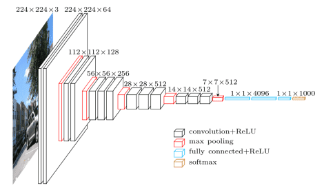
The small filter size of the plethora of convolution filters and the deep architecture of the network outperformed lots of benchmark models of that time. As a result, to this day, VGG16 is considered to be a state-of-the-art model for the ImageNet dataset.
Unfortunately, VGG16 had some major flaws. First, due to the nature of the network, it had several weight parameters. This not only made the models heavier but also increased the inference time for these models.
Understanding the limitations posed by VGG nets, we move on to their spiritual successors; ResNets. Introduced by Kaiming He and Jian Sun, the sheer genius behind the idea of ResNets not only outperformed the VGG nets in many instances, but their architecture enabled a faster inference time as well.
The main idea behind ResNets can be seen in Figure 4.
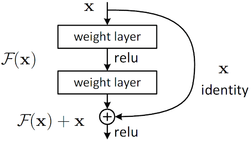
This architecture is termed as “Residual Blocks.” As you can see, the output of a layer not only gets fed to the next layer but also makes a hop and is fed to another layer down the architecture.
Now, this idea right away eliminates the chances of vanishing gradients. But the main idea here is that information from the previous layers is kept alive in the later layers. Hence, an elaborate array of feature maps play a role in adaptively deciding the output of these residual block layers.
ResNet turned out to be a giant leap for the machine learning community. Not only did the results outperform lots of deep architectures at the time of its conception, but ResNet also introduced a whole new direction of how we can make deep architectures better.
With the basic idea of these two models out of the way, let’s jump into the code!
Getting Familiar with Our Dataset
For today’s task, we’ll be using a simple binary classification Dogs & Cats dataset from Kaggle. This 217.78 MB dataset contains 10,000 images of cats and dogs, split in an 80-20 training to test ratio. The training set contains 4000 cat and 4000 dog images, while the test set contains 1000 cat images and 1000 dog images each. There are two reasons for the use of a smaller dataset:
- Fine-tuning our classifier will take less time
- To showcase how fast a pretrained model adapts to a new dataset with less data
Configuring the Prerequisites
To begin with, let’s move into the config.py script stored in the pyimagesearch directory. This script will house the complete training and inference pipeline configuration values.
# import the necessary packages
import torch
import os

# define the parent data dir followed by the training and test paths
BASE_PATH = "dataset"
TRAIN_PATH = os.path.join(BASE_PATH, "training_set")
TEST_PATH = os.path.join(BASE_PATH, "test_set")

# specify ImageNet mean and standard deviation
MEAN = [0.485, 0.456, 0.406]
STD = [0.229, 0.224, 0.225]

# specify training hyperparameters
IMAGE_SIZE = 256
BATCH_SIZE = 128
PRED_BATCH_SIZE = 4
EPOCHS = 15
LR = 0.0001

# determine the device type
DEVICE = torch.device("cuda") if torch.cuda.is_available() else "cpu"

# define paths to store training plot and trained model
PLOT_PATH = os.path.join("output", "model_training.png")
MODEL_PATH = os.path.join("output", "model.pth")
We start by initializing the base training of our dataset on Line 6. Then, on Lines 7 and 8, we use os.path.join to specify our dataset’s training and test folders.
On Lines 11 and 12, we specify the ImageNet mean and standard deviations required later while creating our dataset instances. This is done because the models are pre-trained data preprocessed by these mean and standard deviation values, and we will try to make our present data as similar to the previously trained-on data as we can.
Next, we assign values to hyperparameters like image size, batch size, epochs, etc. (Lines 15-19) and determine the device we will train our models (Line 22).
We end our script by specifying the paths where our training plot and trained model weights will be stored (Lines 25 and 26).
Creating Utility Functions for Our Data Pipeline
We have created some functions to help us in the data pipeline and grouped them in the datautils.py script to better work with our data.
# import the necessary packages
from sklearn.model_selection import train_test_split
from torch.utils.data import DataLoader
from torch.datasets import Subset

def get_dataloader(dataset, batchSize, shuffle=True):
	# create a dataloader
	dl = DataLoader(dataset, batch_size=batchSize, shuffle=shuffle)

	# return the data loader
	return dl
Our first Utility function is the get_dataloader function. It takes the dataset, batch size, and a Boolean variable shuffle as its parameters (Line 6) and returns a PyTorch dataloader instance (Line 11).
def train_val_split(dataset, valSplit=0.2):
	# grab the total size of the dataset
	totalSize = len(dataset)

	# perform training and validation split
	(trainIdx, valIdx) = train_test_split(list(range(totalSize)),
		test_size=valSplit)
	trainDataset = Subset(dataset, trainIdx)
	valDataset = Subset(dataset, valIdx)

	# return training and validation dataset
	return (trainDataset, valDataset)
Next, we create a function called train_val_split, which takes in the dataset and a validation split percentage variable as parameters (Line 13). Since our dataset has only training and test directories, we use the PyTorch dataset subset feature to split the training set into a training and validation set.
We achieve this by first creating indexes for our split using the train_test_split function and then assigning those indexes to the subsets (Lines 20 and 21). This function will return the train and validation data subsets (Line 24).
Creating the Classifier for Our Task
Our next task is to create a classifier for the cats and dogs dataset. Remember that we are not training our called model from scratch but fine-tuning it. For that, we’ll move on to the next script, which is classifier.py.
# import the necessary packages
from torch.nn import Linear
from torch.nn import Module

class Classifier(Module):
	def __init__(self, baseModel, numClasses, model):
		super().__init__()
		# initialize the base model
		self.baseModel = baseModel

		# check if the base model is VGG, if so, initialize the FC
		# layer accordingly
		if model == "vgg":
			self.fc = Linear(baseModel.classifier[6].out_features,
                                numClasses)

		# otherwise, the base model is of type ResNet so initialize
		# the FC layer accordingly
		else:
			self.fc = Linear(baseModel.fc.out_features, numClasses)
In our Classifier module (Line 5), the constructor function takes in the following arguments:
-
baseModel: Since we’ll be calling either the VGG or the ResNet model, we will have already covered the bulk of our architecture. We will plug the called base model directly into our architecture on Line 9. numClasses: Will determine our architecture’s output nodes. For our task, the value is 2.model: A String variable that will tell us if our base model is VGG or a ResNet. Since we have to create a separate output layer specific to our task, we have to take the output of the final linear layer of the models. However, each model has a different method to access the final linear layer. Hence thismodelvariable will help choose the model-specific method accordingly (Line 14 and Line 20).
Notice how for VGGnet, we are using the command baseModel.classifier[6].out_features whereas for ResNet, we are using baseModel.fc.out_features. This is because these models have different named modules and layers. So we have to use different commands to access the last layers of each. Hence, the model variable is very important for our code to work.
	def forward(self, x):
		# pass the inputs through the base model to get the features
		# and then pass the features through of fully connected layer
		# to get our output logits
		features = self.baseModel(x)
		logits = self.fc(features)

		# return the classifier outputs
		return logits
Moving on to the forward function, we simply get the output of the base model on Line 26 and pass it through our final fully connected layer (Line 27) to get the model output.
Training Our Custom Classifier
With the prerequisites out of the way, we move on to train.py. First, we’ll train our classifier to differentiate between cats and dogs.
# USAGE
# python train.py --model vgg
# python train.py --model resnet

# import the necessary packages
from pyimagesearch import config
from pyimagesearch.classifier import Classifier
from pyimagesearch.datautils import get_dataloader
from pyimagesearch.datautils import train_val_split
from torchvision.datasets import ImageFolder
from torchvision.transforms import Compose
from torchvision.transforms import ToTensor
from torchvision.transforms import RandomResizedCrop
from torchvision.transforms import RandomHorizontalFlip
from torchvision.transforms import RandomRotation
from torchvision.transforms import Normalize
from torch.nn import CrossEntropyLoss
from torch.nn import Softmax
from torch import optim
from tqdm import tqdm
import matplotlib.pyplot as plt
import argparse
import torch

# construct the argument parser and parse the arguments
ap = argparse.ArgumentParser()
ap.add_argument("-m", "--model", type=str, default="vgg",
	choices=["vgg", "resnet"], help="name of the backbone model")
args = vars(ap.parse_args())
On Lines 6-23, we have all the required imports for our training module. Unsurprisingly, it’s quite a long list!
For ease of access and choice, we create an argument parser on Line 26, adding the argument model choice (either VGG or ResNet) on Lines 27-29.
The next series of code blocks are very important parts of our project. For example, for fine-tuning a model, we normally freeze the layers of our pre-trained model. However, while ablating different scenarios, we noticed that keeping the convolution layers frozen but the fully connected layers unfreeze for further training have helped our results.
# check if the name of the backbone model is VGG
if args["model"] == "vgg":
	# load VGG-11 model
	baseModel = torch.hub.load("pytorch/vision:v0.10.0", "vgg11",
		pretrained=True, skip_validation=True)

	# freeze the layers of the VGG-11 model
	for param in baseModel.features.parameters():
		param.requires_grad = False
The VGG model architecture called from Torch Hub (Lines 34 and 35) is split into several sub-modules for easier access. The Convolution layers are grouped under a module named features, whereas the following fully connected layers are grouped under a module called classifier. Since we just need to freeze the convolution layers, we directly access the parameters on Line 38 and freeze them by setting requires_grad to False, leaving the classifier module layers untouched.
# otherwise, the backbone model we will be using is a ResNet
elif args["model"] == "resnet":
	# load ResNet 18 model
	baseModel = torch.hub.load("pytorch/vision:v0.10.0", "resnet18",
		pretrained=True, skip_validation=True)

	# define the last and the current layer of the model
	lastLayer = 8
	currentLayer = 1

	# loop over the child layers of the model
	for child in baseModel.children():

		# check if we haven't reached the last layer
		if currentLayer < lastLayer:
			# loop over the child layer's parameters and freeze them
			for param in child.parameters():
				param.requires_grad = False

		# otherwise, we have reached the last layers so break the loop
		else:
			break

		# increment the current layer
		currentLayer += 1
In the case of the base model being ResNet, there are several ways we can approach this. The main thing to remember is that in ResNet, we only have to keep the single last fully connected layer unfrozen. Accordingly, on Lines 48 and 49, we set up the last layer and current layer index.
Looping over the available layers of ResNet on Line 52, we freeze all the layers, except for the last one (Lines 55-65).
# define the transform pipelines
trainTransform = Compose([
	RandomResizedCrop(config.IMAGE_SIZE),
	RandomHorizontalFlip(),
	RandomRotation(90),
	ToTensor(),
	Normalize(mean=config.MEAN, std=config.STD)
])

# create training dataset using ImageFolder
trainDataset = ImageFolder(config.TRAIN_PATH, trainTransform)
We proceed to create the input pipeline, starting with the PyTorch transform instance, which automatically resizes, normalizes, and augments data without much hassle (Lines 68-74).
We top it off by using another great PyTorch utility function called ImageFolder which will automatically create the input and target data, provided the directory is set up correctly (Line 77).
# create training and validation data split
(trainDataset, valDataset) = train_val_split(dataset=trainDataset)

# create training and validation data loaders
trainLoader = get_dataloader(trainDataset, config.BATCH_SIZE)
valLoader = get_dataloader(valDataset, config.BATCH_SIZE)
Using our train_val_split utility function, we split the training dataset into a training and validation set (Line 80). Next, we use the get_dataloader utility function from datautils.py to create our data’s PyTorch dataloader instances (Lines 83 and 84). This will allow us to feed data to our model in a generator-like way seamlessly.
# build the custom model
model = Classifier(baseModel=baseModel.to(config.DEVICE),
	numClasses=2, model=args["model"])
model = model.to(config.DEVICE)

# initialize loss function and optimizer
lossFunc = CrossEntropyLoss()
lossFunc.to(config.DEVICE)
optimizer = optim.Adam(model.parameters(), lr=config.LR)

# initialize the softmax activation layer
softmax = Softmax()
Moving on to our model prerequisites, we create our custom classifier and load it onto our device (Lines 87-89).
We have used cross-entropy as our loss function and Adam optimizer for today’s task (Lines 92-94). In addition, we use a separate softmax loss to help with our training loss additions (Line 97).
# calculate steps per epoch for training and validation set
trainSteps = len(trainDataset) // config.BATCH_SIZE
valSteps = len(valDataset) // config.BATCH_SIZE

# initialize a dictionary to store training history
H = {
	"trainLoss": [],
	"trainAcc": [],
	"valLoss": [],
	"valAcc": []
}
The final step before the training epoch is to set up the training step and validation step values, followed by creating a dictionary that will store all the training history (Lines 100-109).
# loop over epochs
print("[INFO] training the network...")
for epoch in range(config.EPOCHS):
	# set the model in training mode
	model.train()

	# initialize the total training and validation loss
	totalTrainLoss = 0
	totalValLoss = 0

	# initialize the number of correct predictions in the training
	# and validation step
	trainCorrect = 0
	valCorrect = 0
Inside the training loop, we first set our model to training mode (Line 115). Next, we initialize the training loss, validation loss, training, and validation accuracy variables (Lines 118-124).
	# loop over the training set
	for (image, target) in tqdm(trainLoader):
		# send the input to the device
		(image, target) = (image.to(config.DEVICE),
			target.to(config.DEVICE))

		# perform a forward pass and calculate the training loss
		logits = model(image)
		loss = lossFunc(logits, target)

		# zero out the gradients, perform the backpropagation step,
		# and update the weights
		optimizer.zero_grad()
		loss.backward()
		optimizer.step()

		# add the loss to the total training loss so far, pass the
		# output logits through the softmax layer to get output
		# predictions, and calculate the number of correct predictions
		totalTrainLoss += loss.item()
		pred = softmax(logits)
		trainCorrect += (pred.argmax(dim=-1) == target).sum().item()
Looping over the complete training set, we first load the data and target to the device (Lines 129 and 130). Next, we simply pass the data through the model and get the output, followed by plugging the predictions and target into our loss function (Lines 133 and 134),
Lines 138-140 is the standard PyTorch backpropagation step, where we zero out the gradients, perform backpropagation, and update the weights.
Next, we add the loss to our total training loss (Line 145), pass the model output through a softmax to get the isolated prediction value, which we then add to the trainCorrect variable.
	# switch off autograd
	with torch.no_grad():
		# set the model in evaluation mode
		model.eval()

		# loop over the validation set
		for (image, target) in tqdm(valLoader):
			# send the input to the device
			(image, target) = (image.to(config.DEVICE),
				target.to(config.DEVICE))

			# make the predictions and calculate the validation
			# loss
			logits = model(image)
			valLoss = lossFunc(logits, target)
			totalValLoss += valLoss.item()

			# pass the output logits through the softmax layer to get
			# output predictions, and calculate the number of correct
			# predictions
			pred = softmax(logits)
			valCorrect += (pred.argmax(dim=-1) == target).sum().item()
Most of the steps involved in the validation process are the same as the training process, except for a few things:
- The model is set to evaluation mode (Line 152)
- There is no updating of weights
	# calculate the average training and validation loss
	avgTrainLoss = totalTrainLoss / trainSteps
	avgValLoss = totalValLoss / valSteps

	# calculate the training and validation accuracy
	trainCorrect = trainCorrect / len(trainDataset)
	valCorrect = valCorrect / len(valDataset)

	# update our training history
	H["trainLoss"].append(avgTrainLoss)
	H["valLoss"].append(avgValLoss)
	H["trainAcc"].append(trainCorrect)
	H["valAcc"].append(valCorrect)

	# print the model training and validation information
	print(f"[INFO] EPOCH: {epoch + 1}/{config.EPOCHS}")
	print(f"Train loss: {avgTrainLoss:.6f}, Train accuracy: {trainCorrect:.4f}")
	print(f"Val loss: {avgValLoss:.6f}, Val accuracy: {valCorrect:.4f}")
Before exiting the training loop, we calculate the average losses (Lines 173 and 174) and the training and validation accuracy (Lines 177 and 178).
We then proceed to append those values to our training history dictionary (Lines 181-184).
# plot the training loss and accuracy
plt.style.use("ggplot")
plt.figure()
plt.plot(H["trainLoss"], label="train_loss")
plt.plot(H["valLoss"], label="val_loss")
plt.plot(H["trainAcc"], label="train_acc")
plt.plot(H["valAcc"], label="val_acc")
plt.title("Training Loss and Accuracy on Dataset")
plt.xlabel("Epoch #")
plt.ylabel("Loss/Accuracy")
plt.legend(loc="lower left")
plt.savefig(config.PLOT_PATH)

# serialize the model state to disk
torch.save(model.module.state_dict(), config.MODEL_PATH)
Before finishing our training script, we plot all the training dictionary variables (Lines 192-201) and save the figure (Line 202).
Our final task is to save the model weights in the previously defined path (Line 205).
Let’s see how the values per epoch look!
[INFO] training the network...
100%|██████████| 50/50 [01:24<00:00,  1.68s/it]
100%|██████████| 13/13 [00:19<00:00,  1.48s/it]
[INFO] EPOCH: 1/15
Train loss: 0.289117, Train accuracy: 0.8669
Val loss: 0.217062, Val accuracy: 0.9119
100%|██████████| 50/50 [00:47<00:00,  1.05it/s]
100%|██████████| 13/13 [00:11<00:00,  1.10it/s]
[INFO] EPOCH: 2/15
Train loss: 0.212023, Train accuracy: 0.9039
Val loss: 0.223640, Val accuracy: 0.9025
100%|██████████| 50/50 [00:46<00:00,  1.07it/s]
100%|██████████| 13/13 [00:11<00:00,  1.15it/s]
[INFO] EPOCH: 3/15
...
Train loss: 0.139766, Train accuracy: 0.9358
Val loss: 0.187595, Val accuracy: 0.9194
100%|██████████| 50/50 [00:46<00:00,  1.07it/s]
100%|██████████| 13/13 [00:11<00:00,  1.15it/s]
[INFO] EPOCH: 13/15
Train loss: 0.134248, Train accuracy: 0.9425
Val loss: 0.146280, Val accuracy: 0.9437
100%|██████████| 50/50 [00:47<00:00,  1.05it/s]
100%|██████████| 13/13 [00:11<00:00,  1.12it/s]
[INFO] EPOCH: 14/15
Train loss: 0.132265, Train accuracy: 0.9428
Val loss: 0.162259, Val accuracy: 0.9319
100%|██████████| 50/50 [00:47<00:00,  1.05it/s]
100%|██████████| 13/13 [00:11<00:00,  1.16it/s]
[INFO] EPOCH: 15/15
Train loss: 0.138014, Train accuracy: 0.9409
Val loss: 0.153363, Val accuracy: 0.9313
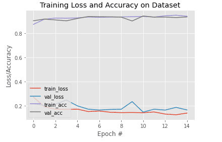
Our pretrained model accuracy is already near 90% in the very first epoch. By the 13th epoch, the values had saturated at about ~94%. To put this in perspective, a pretrained model trained on a different dataset starts at about 86% accuracy on a dataset it hasn’t seen before. That’s how well it has learned to extract features.
A complete overview of the metrics has been plotted in Figure 5.
Putting Our Fine-Tuned Model to the Test
With our model ready for use, we’ll move on to our inference script, inference.py.
# USAGE
# python inference.py --model vgg
# python inference.py --model resnet

# import the necessary packages
from pyimagesearch import config
from pyimagesearch.classifier import Classifier
from pyimagesearch.datautils import get_dataloader
from torchvision.datasets import ImageFolder
from torchvision.transforms import Compose
from torchvision.transforms import ToTensor
from torchvision.transforms import Resize
from torchvision.transforms import Normalize
from torchvision import transforms
from torch.nn import Softmax
from torch import nn
import matplotlib.pyplot as plt
import argparse
import torch
import tqdm

# construct the argument parser and parse the arguments
ap = argparse.ArgumentParser()
ap.add_argument("-m", "--model", type=str, default="vgg",
	choices=["vgg", "resnet"], help="name of the backbone model")
args = vars(ap.parse_args())
Since we’ll have to initialize our model before loading in the weights, we’ll be needing the right model argument. For that, we have created an argument parser on Lines 23-26.
# initialize test transform pipeline
testTransform = Compose([
	Resize((config.IMAGE_SIZE, config.IMAGE_SIZE)),
	ToTensor(),
	Normalize(mean=config.MEAN, std=config.STD)
])

# calculate the inverse mean and standard deviation
invMean = [-m/s for (m, s) in zip(config.MEAN, config.STD)]
invStd = [1/s for s in config.STD]

# define our denormalization transform
deNormalize = transforms.Normalize(mean=invMean, std=invStd)

# create the test dataset
testDataset = ImageFolder(config.TEST_PATH, testTransform)

# initialize the test data loader
testLoader = get_dataloader(testDataset, config.PRED_BATCH_SIZE)
Since we’ll be calculating the accuracy of our model over the complete test data set, we create a PyTorch transform instance for our test data on Lines 29-33.
Consequently, we calculate the inverse mean and inverse standard deviation values, which we use to create a transforms.Normalize instance (Lines 36-40). This is done because the data is preprocessed before getting fed to the model. For display purposes, we have to revert the images to their original state.
Using the ImageFolder utility function, we create our test dataset instance and feed it to the get_dataloader function we had created previously for a test dataLoader instance (Lines 43-46).
# check if the name of the backbone model is VGG
if args["model"] == "vgg":
	# load VGG-11 model
	baseModel = torch.hub.load("pytorch/vision:v0.10.0", "vgg11",
		pretrained=True, skip_validation=True)

# otherwise, the backbone model we will be using is a ResNet
elif args["model"] == "resnet":
	# load ResNet 18 model
	baseModel = torch.hub.load("pytorch/vision:v0.10.0", "resnet18",
		pretrained=True, skip_validation=True)
As mentioned before, since we have to initialize the model again, we check for the model argument given and accordingly use Torch Hub to load the model (Lines 49-58).
# build the custom model
model = Classifier(baseModel=baseModel.to(config.DEVICE),
	numClasses=2, vgg = False)
model = model.to(config.DEVICE)

# load the model state and initialize the loss function
model.load_state_dict(torch.load(config.MODEL_PATH))
lossFunc = nn.CrossEntropyLoss()
lossFunc.to(config.DEVICE)

# initialize test data loss
testCorrect = 0
totalTestLoss = 0
soft = Softmax()
On Lines 61-66, we initialize the model, store it on our device, and load the previously obtained weights during model training.
As we had done in the train.py script, we choose Cross-Entropy as our loss function (Line 67) and initialize the test loss and accuracy (Lines 71 and 72).
# switch off autograd
with torch.no_grad():
	# set the model in evaluation mode
	model.eval()

	# loop over the validation set
	for (image, target) in tqdm(testLoader):
		# send the input to the device
		(image, target) = (image.to(config.DEVICE),
			target.to(config.DEVICE))

		# make the predictions and calculate the validation
		# loss
		logit = model(image)
		loss = lossFunc(logit, target)

		totalTestLoss += loss.item()

		# output logits through the softmax layer to get output
		# predictions, and calculate the number of correct predictions
		pred = soft(logit)
		testCorrect += (pred.argmax(dim=-1) == target).sum().item()
With automatic gradients off (Line 76), we set the model to evaluation mode on Line 78. Then, looping over the test images, we feed them to the model and pass the prediction and targets through the loss function (Lines 81-89).
The accuracy is calculated by passing the predictions through a softmax function (Lines 95 and 96).
# print test data accuracy
print(testCorrect/len(testDataset))

# initialize iterable variable
sweeper = iter(testLoader)

# grab a batch of test data
batch = next(sweeper)
(images, labels) = (batch[0], batch[1])

# initialize a figure
fig = plt.figure("Results", figsize=(10, 10 ))
Now we’ll look at some specific cases of test data and display them. For that reason, we initialize an iterable variable on Line 102 and grab a batch of data (Line 105).
# switch off autograd
with torch.no_grad():
	# send the images to the device
	images = images.to(config.DEVICE)

	# make the predictions
	preds = model(images)

	# loop over all the batch
	for i in range(0, config.PRED_BATCH_SIZE):
		# initialize a subplot
		ax = plt.subplot(config.PRED_BATCH_SIZE, 1, i + 1)

		# grab the image, de-normalize it, scale the raw pixel
		# intensities to the range [0, 255], and change the channel
		# ordering from channels first tp channels last
		image = images[i]
		image = deNormalize(image).cpu().numpy()
		image = (image * 255).astype("uint8")
		image = image.transpose((1, 2, 0))

		# grab the ground truth label
		idx = labels[i].cpu().numpy()
		gtLabel = testDataset.classes[idx]

		# grab the predicted label
		pred = preds[i].argmax().cpu().numpy()
		predLabel = testDataset.classes[pred]

		# add the results and image to the plot
		info = "Ground Truth: {}, Predicted: {}".format(gtLabel,
				predLabel)
		plt.imshow(image)
		plt.title(info)
		plt.axis("off")

	# show the plot
	plt.tight_layout()
	plt.show()
We turn automatic gradients off again and make predictions of the batch of data previously grabbed (Lines 112-117).
Looping over the batch, we grab individual images, denormalize them, rescale them, and fix their dimensions to make them displayable (Lines 127-130).
Based on the image currently under consideration, we first grab its ground truth labels (Lines 133 and 134) and their corresponding predicted labels on Lines 137 and 138 and display them accordingly (Lines 141-145).
Results from Our Fine-Tuned Model
On the overall test dataset, our ResNet-backed custom model yielded an accuracy of 97.5%. In Figures 6-9, we see a batch of data displayed, along with their corresponding ground truth and predicted labels.
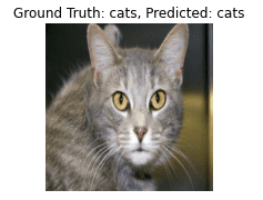

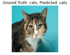
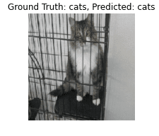
With 97.5% accuracy, you can be assured that this performance level is not just for this batch but for all batches. You can repeatedly run the sweeper variable to get a different data batch to see for yourself.
What's next? We recommend PyImageSearch University.
86+ total classes • 115+ hours hours of on-demand code walkthrough videos • Last updated: May 2026
★★★★★ 4.84 (128 Ratings) • 16,000+ Students Enrolled
I strongly believe that if you had the right teacher you could master computer vision and deep learning.
Do you think learning computer vision and deep learning has to be time-consuming, overwhelming, and complicated? Or has to involve complex mathematics and equations? Or requires a degree in computer science?
That’s not the case.
All you need to master computer vision and deep learning is for someone to explain things to you in simple, intuitive terms. And that’s exactly what I do. My mission is to change education and how complex Artificial Intelligence topics are taught.
If you're serious about learning computer vision, your next stop should be PyImageSearch University, the most comprehensive computer vision, deep learning, and OpenCV course online today. Here you’ll learn how to successfully and confidently apply computer vision to your work, research, and projects. Join me in computer vision mastery.
Inside PyImageSearch University you'll find:
- ✓ 86+ courses on essential computer vision, deep learning, and OpenCV topics
- ✓ 86 Certificates of Completion
- ✓ 115+ hours hours of on-demand video
- ✓ Brand new courses released regularly, ensuring you can keep up with state-of-the-art techniques
- ✓ Pre-configured Jupyter Notebooks in Google Colab
- ✓ Run all code examples in your web browser — works on Windows, macOS, and Linux (no dev environment configuration required!)
- ✓ Access to centralized code repos for all 540+ tutorials on PyImageSearch
- ✓ Easy one-click downloads for code, datasets, pre-trained models, etc.
- ✓ Access on mobile, laptop, desktop, etc.
Summary
Today’s tutorial not only served as a showcase for how you can utilize Torch Hub’s gallery of models, but it also stands as another reminder of how much pre-trained models help us in our daily machine learning escapades.
Imagine if you had to train a big architecture like ResNet from scratch for any task of your choice. It would take much more time and definitely many more epochs. By this point, you surely have to appreciate the idea behind PyTorch Hub to make the whole process of using these state-of-the-art models much more efficient.
Continuing from where we left in our previous week’s tutorial, I would like to emphasize that PyTorch Hub is still rough around the edges, and it still has a huge scope of improvement. Still, surely we are getting closer to the perfect version!
Citation Information
Chakraborty, D. “Torch Hub Series #2: VGG and ResNet,” PyImageSearch, 2021, https://pyimagesearch.com/2021/12/27/torch-hub-series-2-vgg-and-resnet/
@article{dev_2021_THS2,
  author = {Devjyoti Chakraborty},
  title = {{Torch Hub} Series \#2: {VGG} and {ResNet}},
  journal = {PyImageSearch},
  year = {2021},
  note = {https://pyimagesearch.com/2021/12/27/torch-hub-series-2-vgg-and-resnet/},
}
Unleash the potential of computer vision with Roboflow - Free!
- Step into the realm of the future by signing up or logging into your Roboflow account. Unlock a wealth of innovative dataset libraries and revolutionize your computer vision operations.
- Jumpstart your journey by choosing from our broad array of datasets, or benefit from PyimageSearch’s comprehensive library, crafted to cater to a wide range of requirements.
- Transfer your data to Roboflow in any of the 40+ compatible formats. Leverage cutting-edge model architectures for training, and deploy seamlessly across diverse platforms, including API, NVIDIA, browser, iOS, and beyond. Integrate our platform effortlessly with your applications or your favorite third-party tools.
- Equip yourself with the ability to train a potent computer vision model in a mere afternoon. With a few images, you can import data from any source via API, annotate images using our superior cloud-hosted tool, kickstart model training with a single click, and deploy the model via a hosted API endpoint. Tailor your process by opting for a code-centric approach, leveraging our intuitive, cloud-based UI, or combining both to fit your unique needs.
- Embark on your journey today with absolutely no credit card required. Step into the future with Roboflow.
To download the source code to this post (and be notified when future tutorials are published here on PyImageSearch), simply enter your email address in the form below!

Download the Source Code and FREE 17-page Resource Guide
Enter your email address below to get a .zip of the code and a FREE 17-page Resource Guide on Computer Vision, OpenCV, and Deep Learning. Inside you'll find my hand-picked tutorials, books, courses, and libraries to help you master CV and DL!


Comment section
Hey, Adrian Rosebrock here, author and creator of PyImageSearch. While I love hearing from readers, a couple years ago I made the tough decision to no longer offer 1:1 help over blog post comments.
At the time I was receiving 200+ emails per day and another 100+ blog post comments. I simply did not have the time to moderate and respond to them all, and the sheer volume of requests was taking a toll on me.
Instead, my goal is to do the most good for the computer vision, deep learning, and OpenCV community at large by focusing my time on authoring high-quality blog posts, tutorials, and books/courses.
If you need help learning computer vision and deep learning, I suggest you refer to my full catalog of books and courses — they have helped tens of thousands of developers, students, and researchers just like yourself learn Computer Vision, Deep Learning, and OpenCV.
Click here to browse my full catalog.