In this tutorial, you will learn:
- What gradient descent is
- How gradient descent enables us to train neural networks
- Variations of gradient descent, including Stochastic Gradient Descent (SGD)
- How SGD can be improved using momentum and Nesterov acceleration

To learn about gradient descent and its variations, just keep reading.
Gradient Descent Algorithms and Variations
When it comes to training a neural network, gradient descent isn’t just the workhorse — it’s the plow that tills the ground and the farmer that controls where the plow is going.
There have been a tremendous number of variations of gradient descent and optimizers, ranging from your vanilla gradient descent, mini-batch gradient descent, Stochastic Gradient Descent (SGD), and mini-batch SGD, just to name a few.
Furthermore, entirely new model optimizers have been designed with improvements to SGD in mind, including Adam, Adadelta, RMSprop, and others.
Today we are going to review the fundamentals of gradient descent and focus primarily on SGD, including two improvements to SGD, momentum and Nesterov acceleration.
What is gradient descent?
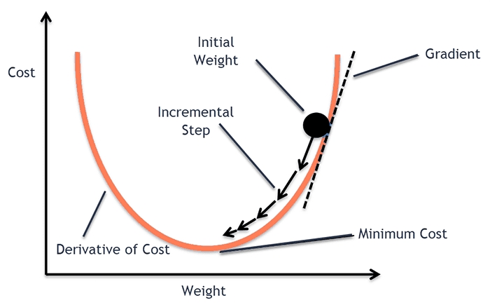
Gradient descent is a first-order optimization algorithm. The goal of gradient descent is to find a local minimum of a differentiable function.
We perform gradient descent iteratively:
- We start by taking our cost/loss function (i.e., the function responsible for computing the value we want to minimize)
- We then compute the gradient of the loss
- And finally, we take a step in the direction opposite of the gradient (since this will take us down the path to our local minimum)
The following figure summarizes gradient descent concisely:
But how does this apply to neural networks and deep learning?
Let’s address that in the next section.
How does gradient descent power neural networks and deep learning?
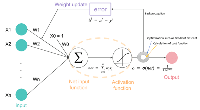
A neural network consists of one or more hidden layers. Each layer consists of a set of parameters. Our goal is to optimize these parameters such that our loss is minimized.
Typical loss functions include binary cross-entropy (two-class classification), categorical cross-entropy (multi-class classification), mean squared error (regression), etc.
There are many types of loss functions, each of which are used in certain roles. Instead of getting too caught up in which loss function is being used, instead think of it this way:
- We initialize our neural network with a random set of weights
- We ask the neural network to make a prediction on a data point from our training set
- We compute the prediction and then the loss/cost function, which tells us how good/bad of a job we did at making the correct prediction
- We compute the gradient off the loss
- And then we ever-so-slightly tweak the parameters of the neural network such that our predictions are better
We do this over and over again until our model is said to “converge” and is able to make reliable, accurate predictions.
There are many types of gradient descent algorithms, but the types we’ll be focusing on here today are:
- Vanilla gradient descent
- Stochastic Gradient Descent (SGD)
- Mini-batch SGD
- SGD with momentum
- SGD with Nesterov acceleration
Vanilla gradient descent
Consider an image dataset of N=10,000 images. Our goal is to train a neural network to classify each of these 10,000 images into a total of T=10 categories.
To train a neural network on this dataset we would utilize gradient descent.
The most basic form of gradient descent, which I like to call vanilla gradient descent, we only update the weights of the network once per update.
What that means is:
- We run all 10,000 images through our network
- We compute the loss and the gradient
- We update the parameters of the network
In vanilla gradient descent we only update the network’s weights once per iteration, meaning that the network sees the entire dataset every time a weight update is performed.
In practice, that’s not very useful.
If the number of training examples is large, then vanilla gradient descent is going to take a long time to converge due to the fact that a weight update is only happening once per data cycle.
Furthermore, the larger your dataset gets, the more nuanced your gradients can become, and if you’re only updating the weights once per epoch then you’re going to be spending the majority of your time computing predictions and not much time actually learning (which is the goal of an optimization problem, right?)
Luckily, there are other variations of gradient descent that address this problem.
Stochastic Gradient Descent (SGD)
Unlike vanilla gradient descent, which only does one weight update per epoch, Stochastic Gradient Descent (SGD) instead does multiple weight updates.
The original formulation of SGD would do N weight updates per epoch where N is equal to the total number of data points in your dataset. So, using our example above, if we have N=10,000 images, then we would have 10,000 weight updates per epoch.
The SGD algorithm becomes:
- Until convergence:
- Randomly select a data point from our dataset
- Make a prediction on it
- Compute the loss and the gradient
- Update the parameters of the network
SGD tends to converge much faster because it’s able to start improving itself after each and every weight update.
That said, performing N weight updates per epoch (where N is equal to the total number of data points in our dataset) is also a bit computationally wasteful — we’ve now swung to the other side of the pendulum.
What we need instead is a median between the two.
Mini-batch SGD
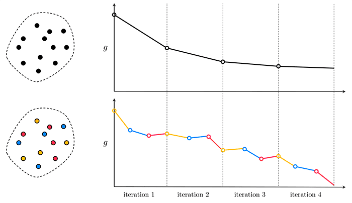
While SGD can converge faster for large datasets, we actually run into another problem — we cannot leverage our vectorized libraries that make training super fast (again, because we are only passing one data point at a time through the network).
There is a variation of SGD called mini-batch SGD that solves this problem. When you hear people talking about SGD what they are almost always referring to is mini-batch SGD.
Mini-batch SGD introduces the concept of a batch size, S. Now, given a dataset of size N, there will be a total of N / S updates to the network.
We can summarize the mini-batch SGD algorithm as:
- Randomly shuffle the input data
- Until convergence:
- Select the next batch of data of size S
- Make predictions on the subset
- Calculate the loss and mean gradient of the mini-batch
- Update the parameters of the network
If you visualize each mini-batch directly then you’ll see a very noisy plot, such as the following one:
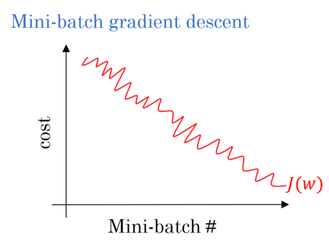
But when you average out the loss across all mini-batches the plot is actually quite stable:
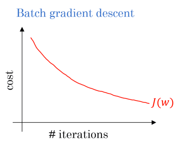
Note: Depending on what deep learning library you are using you may see both types of plots.
When you hear deep learning practitioners talking about SGD they are more than likely talking about mini-batch SGD.
SGD with momentum
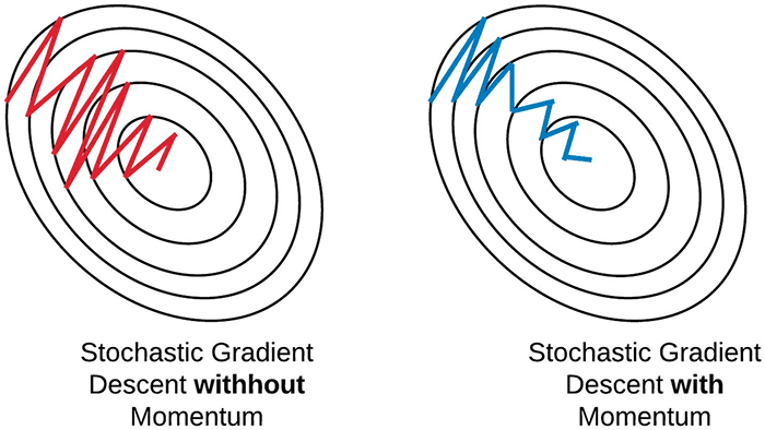
SGD has a problem when navigating areas of the loss landscape that are significantly steeper in one dimension than in others (which you’ll see around local optima).
When this happens, it appears that SGD simply oscillates the ravine instead of descending into areas of lower loss and ideally lower accuracy (see Sebastian Ruder’s excellent article for more details on this phenomenon).
By applying momentum (Figure 6) we build up a head of steam in a direction and then allow gravity to roll us faster and faster down the hill.
Typically you’ll see a momentum value of 0.9 in most SGD applications.
Get used to seeing momentum when using SGD — it is used in the majority of neural network experiments that apply SGD.
SGD with Nesterov acceleration

The problem with momentum is that once you develop a head of steam, the train can easily become out of control and roll right over our local minima and back up the hill again.
Basically, we shouldn’t be blindly following the slope of the gradient.
Nesterov acceleration accounts for this and helps us recognize when the loss landscape starts sloping back up again.
Nearly all deep learning libraries that contain a SGD implementation also include momentum and Nesterov acceleration terms.
Momentum is nearly always a good idea. Nesterov acceleration works in some situations and not in others. You’ll want to treat them as hyperparameters you need to tune when training your neural networks (i.e., pick values for each, run an experiment, log the results, update the parameters, and repeat until you find a set of hyperparameters that yields good results).
What's next? We recommend PyImageSearch University.
86+ total classes • 115+ hours hours of on-demand code walkthrough videos • Last updated: May 2026
★★★★★ 4.84 (128 Ratings) • 16,000+ Students Enrolled
I strongly believe that if you had the right teacher you could master computer vision and deep learning.
Do you think learning computer vision and deep learning has to be time-consuming, overwhelming, and complicated? Or has to involve complex mathematics and equations? Or requires a degree in computer science?
That’s not the case.
All you need to master computer vision and deep learning is for someone to explain things to you in simple, intuitive terms. And that’s exactly what I do. My mission is to change education and how complex Artificial Intelligence topics are taught.
If you're serious about learning computer vision, your next stop should be PyImageSearch University, the most comprehensive computer vision, deep learning, and OpenCV course online today. Here you’ll learn how to successfully and confidently apply computer vision to your work, research, and projects. Join me in computer vision mastery.
Inside PyImageSearch University you'll find:
- ✓ 86+ courses on essential computer vision, deep learning, and OpenCV topics
- ✓ 86 Certificates of Completion
- ✓ 115+ hours hours of on-demand video
- ✓ Brand new courses released regularly, ensuring you can keep up with state-of-the-art techniques
- ✓ Pre-configured Jupyter Notebooks in Google Colab
- ✓ Run all code examples in your web browser — works on Windows, macOS, and Linux (no dev environment configuration required!)
- ✓ Access to centralized code repos for all 540+ tutorials on PyImageSearch
- ✓ Easy one-click downloads for code, datasets, pre-trained models, etc.
- ✓ Access on mobile, laptop, desktop, etc.
Summary
In this tutorial, you learned about gradient and descent and its variations, namely Stochastic Gradient Descent (SGD).
SGD is the workhorse of deep learning. All optimizers, including Adam, Adadelta, RMSprop, etc., have their roots in SGD — each of these optimizers provides tweaks and variations to SGD, ideally improving convergence and making the model more stable during training.
We’ll cover these more advanced optimizers soon, but for the time being, understand that SGD is the basis of all of them.
We can further improve SGD by including a momentum term (nearly always recommended).
Occasionally, Nesterov acceleration can further improve SGD (dependent on your specific project).
To download the source code to this post (and be notified when future tutorials are published here on PyImageSearch), simply enter your email address in the form below!

Join the PyImageSearch Newsletter and Grab My FREE 17-page Resource Guide PDF
Enter your email address below to join the PyImageSearch Newsletter and download my FREE 17-page Resource Guide PDF on Computer Vision, OpenCV, and Deep Learning.

Comment section
Hey, Adrian Rosebrock here, author and creator of PyImageSearch. While I love hearing from readers, a couple years ago I made the tough decision to no longer offer 1:1 help over blog post comments.
At the time I was receiving 200+ emails per day and another 100+ blog post comments. I simply did not have the time to moderate and respond to them all, and the sheer volume of requests was taking a toll on me.
Instead, my goal is to do the most good for the computer vision, deep learning, and OpenCV community at large by focusing my time on authoring high-quality blog posts, tutorials, and books/courses.
If you need help learning computer vision and deep learning, I suggest you refer to my full catalog of books and courses — they have helped tens of thousands of developers, students, and researchers just like yourself learn Computer Vision, Deep Learning, and OpenCV.
Click here to browse my full catalog.