Table of Contents
- Integrating Streamlit with Snowflake for Live Cloud Data Apps (Part 2)
-
Building the Main Driver Script
- Imports and Page Setup
- Connection Page: Detecting Environment Variables and Validating Configuration
- Run Query: Executing Read-Only SQL with Timing and Row Limits
- Explore Data: Previewing and Summarizing Query Results
- Visualize: Creating Charts from Query Results
- Blend Data: Combining Snowflake Tables with Local Datasets
- Export: Downloading Query Results
- Performance and Caching: Making Queries Efficient
- Summary
Integrating Streamlit with Snowflake for Live Cloud Data Apps (Part 2)
Continued from Part 1.
This lesson is part of a series on Streamlit Apps:
- Getting Started with Streamlit: Learn Widgets, Layouts, and Caching
- Building Your First Streamlit App: Uploads, Charts, and Filters (Part 1)
- Building Your First Streamlit App: Uploads, Charts, and Filters (Part 2)
- Integrating Streamlit with Snowflake for Live Cloud Data Apps (Part 1)
- Integrating Streamlit with Snowflake for Live Cloud Data Apps (Part 2) (this tutorial)
To learn how to query, visualize, and export live warehouse data from Streamlit, just keep reading.
Building the Main Driver Script
Now that we’ve prepared our helper modules and configured Snowflake credentials, it’s time to bring everything together into one cohesive Streamlit app. The main driver script, lesson3_main.py, acts as the command center — defining layout, navigation, and page logic. It connects Streamlit’s interactive UI to the Snowflake data warehouse and orchestrates how users query, explore, visualize, and export results.
This file follows the same philosophy as previous lessons: start lightweight, keep functionality modular, and build progressively. By the end, you’ll have a fully functional dashboard that can read live data from Snowflake, cache expensive queries, and even blend them with local datasets such as the Iris sample.

Imports and Page Setup
The first few lines of lesson3_main.py set the tone for the entire app. Here’s the opening block:
from __future__ import annotations
import streamlit as st
import pandas as pd
from pyimagesearch import (
    settings,
    load_iris_sample,
    iris_feature_scatter,
)
import time
import re
We begin with a docstring that clearly describes the lesson’s purpose and a simple run command — a helpful reminder for future readers. The from __future__ import annotations line ensures type hints are treated as strings, improving performance and avoiding circular imports when referencing types.
Next come the core imports:
streamlitfor the web interfacepandasfor tabular data manipulationsettings,load_iris_sample, andiris_feature_scatterfrom ourpyimagesearchpackage, connecting this lesson to earlier utility modulestimeandrefor lightweight timing and SQL pattern matching, respectively
Then, we configure the overall page layout:
st.set_page_config(page_title="Lesson 3 - Snowflake Integration", layout="wide")
st.title("❄️ Lesson 3: Streamlit + Snowflake Data Apps")
st.write(
    "We connect to Snowflake, run parameterized queries, and blend remote + local data."
)
st.set_page_config must always appear near the top of a Streamlit script — it defines the page title (visible in the browser tab) and a wide layout so your tables and charts can stretch comfortably across the screen. The emoji in the title isn’t just playful — it adds scannability and aligns visually with earlier lessons.
The short description (st.write) summarizes the app’s goal in one line: connecting, querying, and blending Snowflake data.
Finally, we import our Snowflake helper functions lazily:
try:
    from pyimagesearch.snowflake_utils import SnowflakeCredentials, run_query
except Exception as e:  # pragma: no cover
    SnowflakeCredentials = None  # type: ignore
    run_query = None  # type: ignore
This “lazy import” pattern ensures earlier lessons can still run even if the snowflake-connector-python package isn’t installed. Instead of failing immediately, it defers dependency errors until the user actually visits a Snowflake-dependent page. That keeps the development environment clean and modular.
After setting up the title and page layout, we define the sidebar navigation — the central control panel for moving between app sections:
st.sidebar.title("Sections")
section = st.sidebar.radio(
    "Go to",
    [
        "Connection",
        "Run Query",
        "Explore Data",
        "Visualize",
        "Blend Data",
        "Export",
        "Performance",
    ],
)
st.sidebar.caption("Lesson 3 demo app (extended)")
This radio button acts as the main menu. Each option corresponds to a page in the app, guiding the user step by step — from testing the connection to exporting results. Because Streamlit reruns the script top-to-bottom on every interaction, the selected section value controls which code block is executed next. The small caption underneath adds context, reminding readers that this is the extended demo version used in Lesson 3.

Next come a few compact helper functions that keep our code clean and readable:
def snowflake_available() -> bool:
    return settings.snowflake_enabled and run_query is not None
This function is a quick diagnostic switch: it checks whether the Snowflake credentials exist and whether the connector import succeeded. Having this centralized means we don’t repeat the same conditional logic throughout the app.
You might notice it appears twice in the source file — that’s simply a duplicate definition left in for compatibility while refactoring; it doesn’t affect behavior since both versions return the same condition.
The _build_creds() function consolidates how credentials are passed into the Snowflake connector:
def _build_creds():  # helper to avoid repetition
    return SnowflakeCredentials(  # type: ignore
        user=settings.snowflake_user,  # type: ignore
        password=settings.snowflake_password,  # type: ignore
        account=settings.snowflake_account,  # type: ignore
        warehouse=settings.snowflake_warehouse,  # type: ignore
        database=settings.snowflake_database,  # type: ignore
        schema=settings.snowflake_schema,  # type: ignore
        role=settings.snowflake_role,
    )
Without this wrapper, every page that queries Snowflake would need to rewrite the same long argument list. Centralizing the credential construction ensures consistency and makes it easy to modify later (e.g., if you add MFA (multi-factor authentication) tokens or session parameters).
Finally, the _read_only() helper function enforces a lightweight SQL safety check:
def _read_only(sql: str) -> bool:
    # simplistic guard to discourage destructive statements in demo context
    destructive = re.compile(r"\b(UPDATE|DELETE|INSERT|MERGE|ALTER|DROP|TRUNCATE)\b", re.I)
    return not destructive.search(sql)
This function uses a simple regular expression to detect potentially destructive commands (e.g., DELETE, ALTER, or DROP). If any of these appear in the SQL (Structured Query Language) string, the function returns False, blocking the query. It’s not meant to replace a real SQL firewall, but it prevents accidental table modifications during experimentation.
In production, you’d complement this with parameterized queries or stored procedures for full protection.

DELETE, UPDATE, DROP), ensuring only safe queries are executed against Snowflake in the demo environment (source: image by the author).Connection Page: Detecting Environment Variables and Validating Configuration
The Connection section is the very first stop in the sidebar. It serves a simple but crucial purpose: verifying that your Snowflake credentials are correctly loaded and that the app is ready to query the warehouse.
Here’s the corresponding block from the script:
if section == "Connection":
    st.header("Snowflake Connection Status")
    if snowflake_available():
        st.success("Environment variables detected. Ready to query.")
        if st.checkbox("Show loaded settings", False):
            st.json(
                {
                    "account": settings.snowflake_account,
                    "warehouse": settings.snowflake_warehouse,
                    "database": settings.snowflake_database,
                    "schema": settings.snowflake_schema,
                    "role": settings.snowflake_role,
                }
            )
    else:
        st.error("Snowflake not fully configured.")
        st.markdown(
            "Set SNOWFLAKE_* environment variables (see README) and install dependencies."
        )
We start by checking which page the user has selected in the sidebar. If it’s Connection, the app displays a header labeled Snowflake Connection Status.
The first conditional — if snowflake_available() — runs the helper function we defined earlier. It ensures two things:
- All required Snowflake credentials are available (i.e.,
user,password,account,warehouse,database, andschema) - The Snowflake connector (
run_query) was successfully imported
If both checks pass, Streamlit displays a reassuring green success banner:
✅ Environment variables detected. Ready to query.
This immediate feedback tells users their secrets are properly configured. A checkbox labeled “Show loaded settings” optionally reveals the non-sensitive fields (e.g., account, warehouse, database, schema, and role) in JSON format. Passwords and usernames remain hidden for security, but these values help verify that the correct Snowflake environment is being used.
If credentials are missing, the app displays an error state with a clear next step:
❌ Snowflake not fully configured.
Set SNOWFLAKE_* environment variables (see README) and install dependencies.
This message guides users to ensure their .streamlit/secrets.toml or environment variables are correctly set — no guesswork required.

account, warehouse, database, schema, and role). The interface confirms readiness to query data directly from Snowflake using Streamlit’s interactive dashboard (source: image by the author).This page may look simple, but it’s essential for debugging the environment setup. Before running any SQL, you confirm that Streamlit can detect your Snowflake credentials.
With a verified connection in place, the next step is where the real action begins — executing live SQL queries against Snowflake.
Run Query: Executing Read-Only SQL with Timing and Row Limits
Once your connection is verified, the next logical step is to run SQL queries against Snowflake. This page lets you enter custom SQL commands, execute them securely, preview the results, and measure query performance — all from within Streamlit.
Here’s the relevant block:
elif section == "Run Query":
    st.header("Run Query (Read‑Only Guard)")
    if not snowflake_available():
        st.warning("Snowflake not configured.")
    else:
        creds = _build_creds()
        default_query = "SELECT CURRENT_TIMESTAMP() AS now;"
        sql = st.text_area("SQL", value=default_query, height=160)
        col_run, col_lim = st.columns([1, 2])
        max_rows = col_lim.number_input("Client row cap (preview)", 10, 5000, 200)
        if col_run.button("Execute", type="primary"):
            if not _read_only(sql):
                st.error("Destructive statements blocked in demo.")
            else:
                # Ensure a LIMIT is present for huge accidental scans (basic heuristic)
                if "limit" not in sql.lower():
                    sql_display = sql + f"\n-- (Client-side preview capped to {max_rows} rows)"
                else:
                    sql_display = sql
                with st.spinner("Running query..."):
                    start = time.time()
                    try:
                        df = run_query(creds, sql)  # type: ignore
                    except Exception as e:  # noqa: BLE001
                        st.error(f"Query failed: {e}")
                    else:
                        elapsed = time.time() - start
                        st.success(f"Returned {len(df)} rows in {elapsed:.2f}s")
                        st.caption(sql_display)
                        st.dataframe(df.head(int(max_rows)))
                        st.session_state.query_df = df
                        # rudimentary history
                        history = st.session_state.get("query_history", [])
                        history.append({"sql": sql[:200], "rows": len(df), "time": elapsed})
                        st.session_state.query_history = history[-10:]
        if st.checkbox("Show last query history"):
            for item in st.session_state.get("query_history", []):
                st.code(f"{item['rows']} rows | {item['time']:.2f}s\n{item['sql']}")
After setting the header, the app checks snowflake_available() again — if credentials aren’t configured, it displays a neutral warning rather than failing outright.
Next, we call the _build_creds() function to instantiate a SnowflakeCredentials object using the secure values we stored earlier. The default query is a harmless one:
SELECT CURRENT_TIMESTAMP() AS now;
This is a quick way to test that your Snowflake warehouse is live and responsive.
The user-facing input is provided by st.text_area, which allows you to enter any SQL statement. The height=160 ensures there’s enough space for multi-line queries.
Below that, two columns organize controls neatly:
- A Run button on the left, labeled “Execute.”
- A number input on the right, limiting the maximum number of rows to display (Client row cap).
This row limit serves as a browser safety mechanism — Snowflake tables can be massive, and rendering tens of thousands of rows in Streamlit could freeze the interface.
When the Execute button is clicked, the code first checks the _read_only(sql) helper to ensure the command isn’t destructive. Any SQL containing UPDATE, DELETE, ALTER, or similar keywords is immediately blocked with a red error message.
If it passes the guard, the query runs inside a spinner block:
with st.spinner("Running query..."):
    start = time.time()
    ...
The spinner provides instant visual feedback while the query executes. Using the time.time() function, we measure and display the elapsed time once the results return. The preview is then rendered with st.dataframe(df.head(int(max_rows))), capped at the selected row limit.
At the same time, the DataFrame is stored in st.session_state.query_df, allowing other pages (e.g., Explore Data or Visualize) to access it without re-running the query. This simple session-state trick turns your single-page app into a multi-step data workflow.
Lastly, we maintain a small query history buffer:
history = st.session_state.get("query_history", [])
history.append({"sql": sql[:200], "rows": len(df), "time": elapsed})
st.session_state.query_history = history[-10:]
This stores the last 10 executed queries, along with their row counts and execution times. A checkbox labeled “Show last query history” lets you view this list, formatted with st.code for readability.
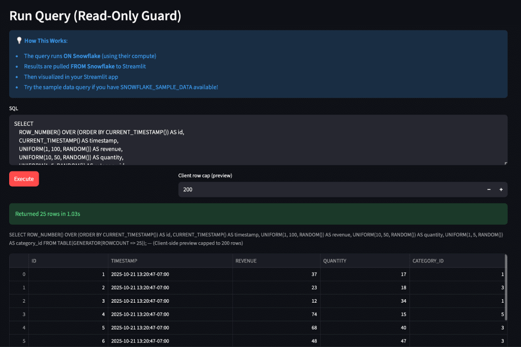
This section is the first point where your app truly talks to Snowflake — running live SQL and returning a Pandas DataFrame.
With the query results stored in session state, you’re now ready to explore and analyze the returned data visually.
Explore Data: Previewing and Summarizing Query Results
After running your first query, it’s time to inspect and understand the data you just pulled from Snowflake. The Explore Data section provides a clean, interactive view that helps you quickly validate your query output before moving on to charts or blending operations.
Here’s the corresponding block from the code:
elif section == "Explore Data":
    st.header("Explore Last Result Set")
    df = st.session_state.get("query_df")
    if df is None:
        st.info("Run a query first in 'Run Query'.")
    else:
        col1, col2, col3 = st.columns(3)
        col1.metric("Rows", len(df))
        col2.metric("Columns", df.shape[1])
        col3.metric("Null Cells", int(df.isna().sum().sum()))
        st.subheader("Preview")
        preview_mode = st.radio("View", ["Head", "Tail", "Sample"], horizontal=True)
        if preview_mode == "Head":
            st.dataframe(df.head())
        elif preview_mode == "Tail":
            st.dataframe(df.tail())
        else:
            st.dataframe(df.sample(min(5, len(df))))
        with st.expander("Describe / Summary", expanded=False):
            try:
                st.dataframe(df.describe(include="all").transpose())
            except Exception:
                st.warning("Describe failed for this dataset (mixed or non-numeric heavy).")
Let’s walk through this.
The page begins with the header “Explore Last Result Set.” The app immediately tries to retrieve the DataFrame stored in st.session_state.query_df. This variable holds the most recent successful query result from the previous section.
If the user hasn’t executed any queries yet, the app displays a friendly informational message:
ℹ️ Run a query first in “Run Query.”
This prevents errors while keeping the flow intuitive.
Once a DataFrame is available, three key metrics appear at the top (i.e., Rows, Columns, and Null Cells). Each one uses the st.metric widget from Streamlit to render a compact metric. These instant stats help you validate the data size and completeness before deeper analysis.
Next, we show a preview section. Users can toggle between:
Head: displays the first few rows,Tail: shows the last few rows,Sample: picks a random handful of rows (great for large datasets).
This small radio control gives you quick views of different parts of your dataset, ensuring you don’t miss anomalies at the start or end of the results.
The real highlight is the “Describe / Summary” expander below. Inside it, we compute descriptive statistics using df.describe(include="all"), transposing the result so that each column appears as a row. This is perfect for mixed datasets that contain both numeric and categorical fields.
We wrap this section in a try/except to gracefully handle edge cases — for example, if the dataset contains complex objects or nested types that pandas.describe() can’t summarize. Instead of crashing, Streamlit will show:
⚠️ Describe failed for this dataset (mixed or non-numeric heavy).
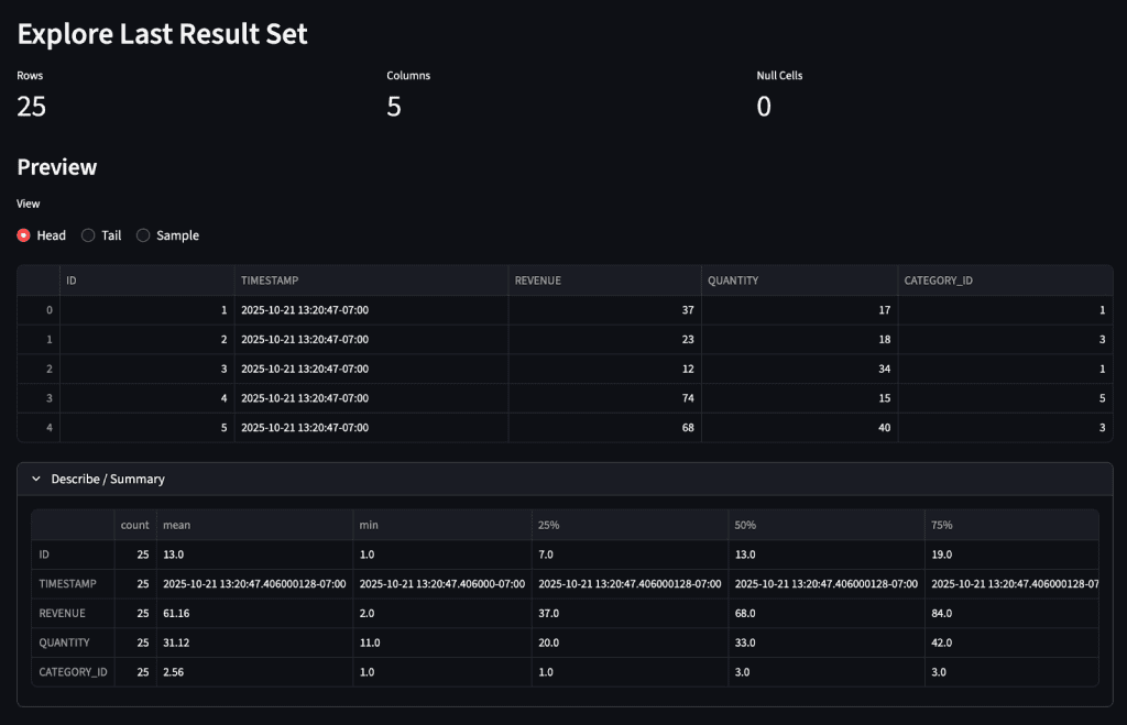
revenue, quantity, and category_id), enabling instant validation of retrieved data (source: image by the author).This section effectively acts as your data validation checkpoint. You confirm that the query results look correct, assess data quality (missing values, column count), and sample your records without leaving the app.
Once you’re confident that the results make sense, you can move forward to visualize them using charts and graphs.
Visualize: Creating Charts from Query Results
Once you’ve verified the data in your Explore section, the next logical step is to visualize it. The Visualize page transforms the raw Snowflake query output into interactive charts, helping you spot patterns, trends, and anomalies at a glance.
Here’s the relevant code block:
elif section == "Visualize":
    st.header("Visualize Query Results")
    df = st.session_state.get("query_df")
    if df is None or df.empty:
        st.info("Run a query first.")
    else:
        numeric_cols = df.select_dtypes(include=["number"]).columns.tolist()
        if not numeric_cols:
            st.warning("No numeric columns available for plotting.")
        else:
            chart_type = st.selectbox("Chart Type", ["Line", "Bar", "Scatter", "Histogram"])
            if chart_type in {"Line", "Bar"}:
                col = st.selectbox("Column", numeric_cols)
                if chart_type == "Line":
                    st.line_chart(df[col])
                else:
                    st.bar_chart(df[col])
            elif chart_type == "Scatter":
                x = st.selectbox("X", numeric_cols)
                y = st.selectbox("Y", numeric_cols)
                st.scatter_chart(df[[x, y]])
            elif chart_type == "Histogram":
                import matplotlib.pyplot as plt  # local import to avoid overhead if unused
                col = st.selectbox("Column", numeric_cols)
                fig, ax = plt.subplots()
                df[col].hist(ax=ax, bins=30, color="#4b8bbe", edgecolor="black")
                ax.set_title(f"Histogram of {col}")
                st.pyplot(fig)
The page opens with the header “Visualize Query Results” and immediately attempts to load the last queried DataFrame from st.session_state.query_df. If no data is available, an informational prompt reminds the user to “Run a query first.”
Next, we identify all numeric columns in the dataset using:
numeric_cols = df.select_dtypes(include=["number"]).columns.tolist()
This ensures that only quantitative data is used for plotting — since chart types (e.g., line, bar, scatter, or histogram) require numerical axes.
If no numeric columns are detected (e.g., if your result only contains text fields), Streamlit warns:
⚠️ No numeric columns available for plotting.
Otherwise, users can select from four chart types using a dropdown menu (st.selectbox): Line, Bar, Scatter, and Histogram.
Each option dynamically updates the chart controls:
- Line / Bar: requests a single numeric column to plot over its index
- Scatter: requires both
XandYaxes - Histogram: uses Matplotlib to render a distribution view of a single column
This structure is simple but powerful — it provides a basic analytics layer without external dashboards or front-end code.
Note how the Matplotlib import is performed inside the Histogram branch:
import matplotlib.pyplot as plt
This lazy import avoids unnecessary overhead when users don’t select that chart type, keeping the app lightweight.
Each chart is rendered inline using Streamlit’s native plotting APIs (e.g., st.line_chart(), st.bar_chart(), and st.scatter_chart()). These functions are optimized for fast reactivity, redrawing immediately whenever the user switches columns or chart types.
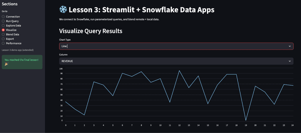
This section gives your app a visual analytics layer — turning query results into insights with minimal code. You’ve now gone from connection setup to exploration to visualization — all in a single, consistent Streamlit workflow.
Next, we’ll bridge the two worlds by combining Snowflake data with a local dataset, showing how to blend and compare sources seamlessly.
Blend Data: Combining Snowflake Tables with Local Datasets
Now that you’ve run queries and visualized results, it’s time to see how Streamlit can mix live warehouse data with local files. This section demonstrates how to “blend” Snowflake tables with a small CSV dataset (the Iris sample you’ve been using since Lesson 1).
Here’s the relevant code block:
elif section == "Blend Data":
    st.header("Blend Local + Remote Data")
    base_df = load_iris_sample(settings.default_sample_path)
    st.write("Local sample (Iris subset):", base_df.shape)
    if snowflake_available():
        st.write("Attempting small Snowflake sample query (replace with a real table).")
        example_table = st.text_input("Snowflake table (must exist)", "YOUR_TABLE")
        if st.button("Fetch & Blend"):
            try:
                creds = SnowflakeCredentials(
                    user=settings.snowflake_user,  # type: ignore
                    password=settings.snowflake_password,  # type: ignore
                    account=settings.snowflake_account,  # type: ignore
                    warehouse=settings.snowflake_warehouse,  # type: ignore
                    database=settings.snowflake_database,  # type: ignore
                    schema=settings.snowflake_schema,  # type: ignore
                    role=settings.snowflake_role,
                )
                snow_df = run_query(creds, f"SELECT * FROM {example_table} LIMIT 50")  # type: ignore
            except Exception as e:
                st.error(f"Failed: {e}")
            else:
                st.success(f"Remote shape: {snow_df.shape}")
                st.dataframe(snow_df.head())
                st.write("(You would now perform joins / merges depending on domain.)")
    else:
        st.info("Configure Snowflake to enable blending example.")
The section starts by loading your local dataset, using the same helper function introduced earlier:
base_df = load_iris_sample(settings.default_sample_path)
A simple st.write call displays its shape, reminding you that this small Iris CSV serves as your on-disk data source. This local dataset provides a sandbox for testing data-merge patterns without any cost or network dependency.
Next, the app checks if a Snowflake connection is available. If credentials are set up correctly, a prompt appears:
"Attempting small Snowflake sample query (replace with a real table)."
The user then enters a table name via a text input box (st.text_input). This could be any accessible table, such as:
SNOWFLAKE_SAMPLE_DATA.TPCH_SF1.CUSTOMER
When the Fetch & Blend button is pressed, the app rebuilds Snowflake credentials and executes a limited query (SELECT * ... LIMIT 50) to fetch a small subset of rows. The results are shown instantly with st.dataframe(snow_df.head()), along with a success message indicating the shape of the remote dataset.
This sample step mimics how you would later join warehouse data with your local experiment results. In a production workflow, you might merge two DataFrames with pd.merge() or concatenate results from multiple queries to create unified analytics tables.
If Snowflake credentials aren’t configured, Streamlit gracefully displays:
"Configure Snowflake to enable blending example."
No crashes, no stack traces — just a clear hint that you need to finish setup first.
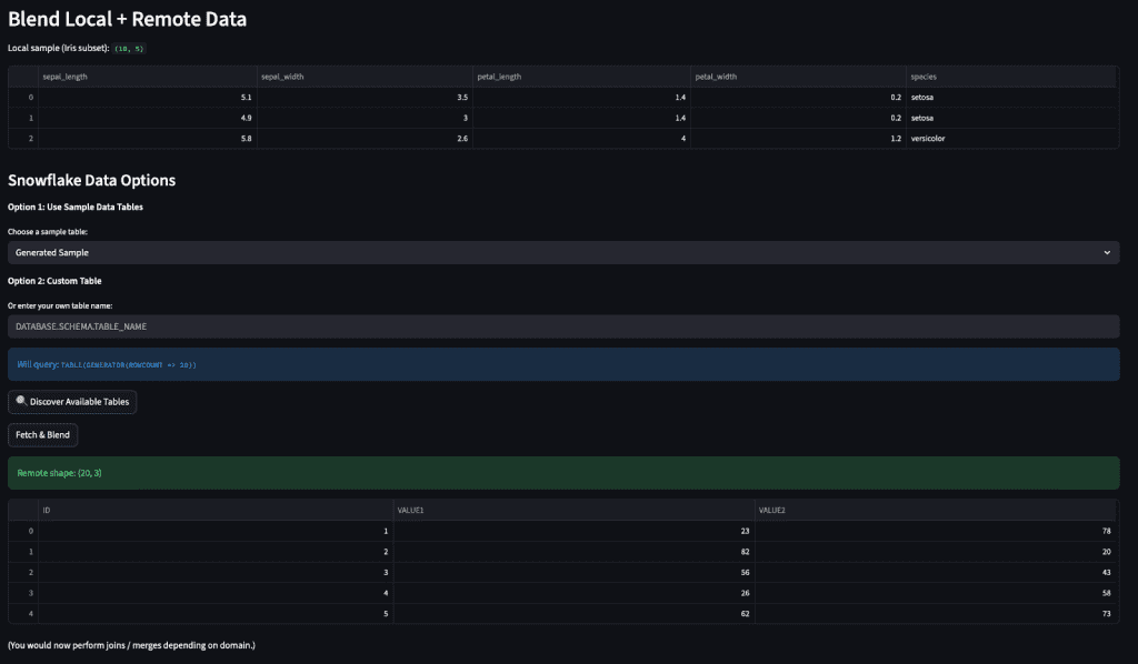
This page completes your app’s data lifecycle loop: you can now connect to a warehouse, query live data, explore and visualize it, and even combine it with local context or model outputs — all without leaving Streamlit.
Next, we’ll make that data portable with the Export section, where users can download their query results as CSV files for external analysis or sharing.
Export: Downloading Query Results
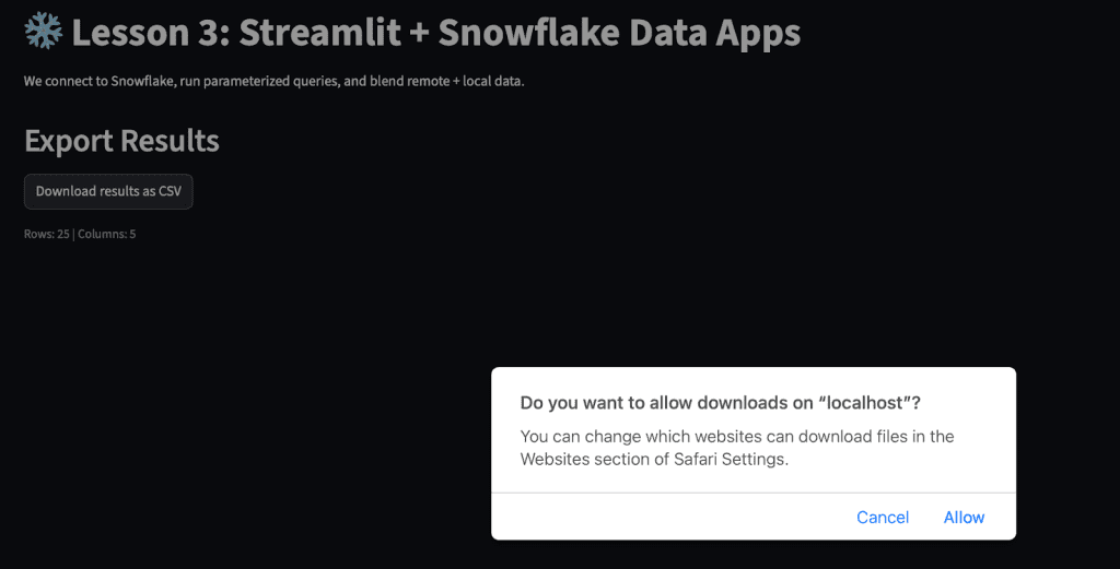
Once users have explored, visualized, or even blended their datasets, the final step is to make the data portable. The Export page provides a simple, frictionless way to download the last query’s output as a CSV file — no extra code, no manual file handling.
Here’s the corresponding block of code:
elif section == "Export":
    st.header("Export Results")
    df = st.session_state.get("query_df")
    if df is None or df.empty:
        st.info("No results to export yet.")
    else:
        st.download_button(
            "Download results as CSV",
            df.to_csv(index=False).encode("utf-8"),
            file_name="query_results.csv",
            mime="text/csv",
        )
        st.caption(f"Rows: {len(df)} | Columns: {df.shape[1]}")
Let’s break it down.
The app begins by retrieving the stored DataFrame from st.session_state.query_df. This ensures users don’t have to rerun a query to download results — Streamlit automatically keeps the last executed query’s data in memory.
If there’s no DataFrame available (perhaps the user hasn’t executed any query yet), an informational message appears:
ℹ️ “No results to export yet.”
Otherwise, the app uses Streamlit’s built-in st.download_button to convert the DataFrame into a downloadable CSV stream.
The logic is elegantly simple:
df.to_csv(index=False).encode("utf-8")
This generates a UTF-8 encoded CSV without the DataFrame’s index column, ensuring compatibility with most spreadsheet tools (e.g., Excel, Google Sheets, or Pandas reimports).
The file is automatically named query_results.csv, but you can easily change this if you want to append timestamps or dynamic identifiers. The MIME type text/csv ensures browsers treat it as a text file for download.
Finally, a small caption displays basic context:
Rows: 50 | Columns: 8
This confirmation reassures users that they’re exporting the expected data — especially useful when handling multiple datasets in one session.
This section completes the data lifecycle for your app: you can now connect, query, visualize, combine, and export — all in one seamless Streamlit experience.
In the final section, you’ll learn how to keep things fast and efficient with Streamlit’s caching, ensuring that repeated queries return instantly without hitting the warehouse each time.
Performance and Caching: Making Queries Efficient
By this point, your Streamlit app can connect to Snowflake, run queries, explore data, visualize it, and export results. But one problem remains: repeated queries can slow down your app and unnecessarily consume compute credits.
This section introduces caching — a simple way to reuse results for recurring queries without re-hitting Snowflake each time.
Here’s the code snippet:
elif section == "Performance":
    st.header("Performance & Caching Demo")
    if not snowflake_available():
        st.info("Configure Snowflake to demonstrate remote caching.")
    else:
        creds = _build_creds()

        @st.cache_data(ttl=600)
        def cached_query(sql: str):  # simple wrapper for demonstration
            return run_query(creds, sql)  # type: ignore

        sql = st.text_input("Stable dimension query (will be cached)", "SELECT CURRENT_DATE AS d;")
        if st.button("Run (cached)"):
            start = time.time()
            try:
                df = cached_query(sql)
            except Exception as e:  # noqa: BLE001
                st.error(f"Failed: {e}")
            else:
                st.success(f"Rows: {len(df)} | Elapsed: {time.time() - start:.3f}s (cached on repeat)")
                st.dataframe(df)
        if st.button("Clear Cache"):
            cached_query.clear()
            st.info("Cache cleared.")
The section begins by checking if Snowflake is configured. If it’s not, the app gently informs users that they need to set up credentials before caching can be demonstrated.
If Snowflake is available, the app builds credentials using _build_creds() and defines a small inner function decorated with Streamlit’s caching mechanism:
@st.cache_data(ttl=600)
def cached_query(sql: str):  # simple wrapper for demonstration
    return run_query(creds, sql)  # type: ignore
This decorator stores the query results in memory (and on disk) for 600 seconds (10 minutes). During that period, any repeated call to the same SQL query will instantly return the cached DataFrame instead of making another round trip to Snowflake.
The ttl (time-to-live) argument is critical — it ensures cached data eventually expires, preventing stale results. For fast-changing tables, you might set it to 60 seconds; for dimension tables that rarely change, 3600 seconds (1 hour) is common.
The next part defines a text input for a simple SQL statement and two buttons:
- Run (cached): executes the query (or retrieves from cache if previously run)
- Clear Cache: resets all cached data, forcing a fresh query on the next run
Each execution measures elapsed time with:
start = time.time()
and then reports:
Rows: 1 | Elapsed: 0.045s (cached on repeat)
On first execution, the query takes the normal Snowflake round-trip time (usually around 1 second). On subsequent runs, it completes almost instantly, confirming caching is working.
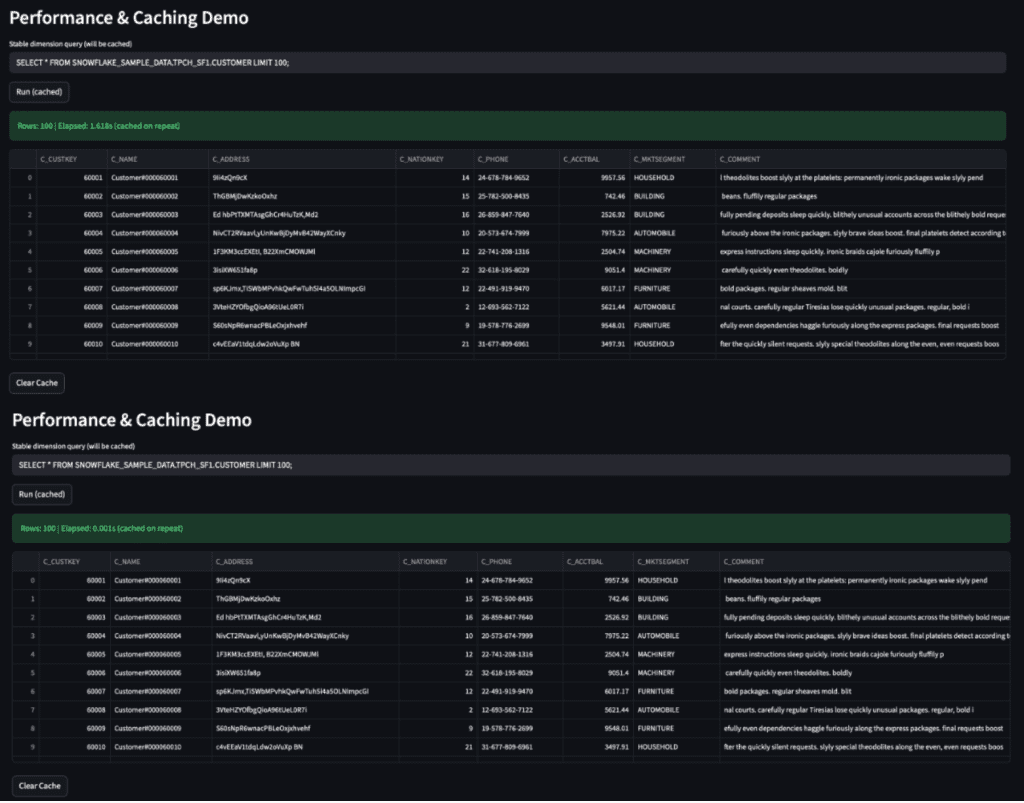
SELECT * FROM SNOWFLAKE_SAMPLE_DATA.TPCH_SF1.CUSTOMER LIMIT 100;) and showcases how caching improves efficiency. The first run takes approximately 1.6 seconds, while subsequent runs retrieve results instantly (0.001s), demonstrating the seamless integration of Snowflake and Streamlit for fast, cached query performance (source: image by the author).This simple caching layer dramatically improves responsiveness, especially for dashboards that query the same data repeatedly (e.g., daily summaries or static lookup tables). It also reduces warehouse costs by minimizing redundant compute.
With this final section, your Streamlit + Snowflake app is now feature-complete — secure, performant, and ready for internal analytics use.
Next, we’ll wrap up the lesson with a summary and clear next steps toward production-ready apps.
What's next? We recommend PyImageSearch University.
86+ total classes • 115+ hours hours of on-demand code walkthrough videos • Last updated: March 2026
★★★★★ 4.84 (128 Ratings) • 16,000+ Students Enrolled
I strongly believe that if you had the right teacher you could master computer vision and deep learning.
Do you think learning computer vision and deep learning has to be time-consuming, overwhelming, and complicated? Or has to involve complex mathematics and equations? Or requires a degree in computer science?
That’s not the case.
All you need to master computer vision and deep learning is for someone to explain things to you in simple, intuitive terms. And that’s exactly what I do. My mission is to change education and how complex Artificial Intelligence topics are taught.
If you're serious about learning computer vision, your next stop should be PyImageSearch University, the most comprehensive computer vision, deep learning, and OpenCV course online today. Here you’ll learn how to successfully and confidently apply computer vision to your work, research, and projects. Join me in computer vision mastery.
Inside PyImageSearch University you'll find:
- ✓ 86+ courses on essential computer vision, deep learning, and OpenCV topics
- ✓ 86 Certificates of Completion
- ✓ 115+ hours hours of on-demand video
- ✓ Brand new courses released regularly, ensuring you can keep up with state-of-the-art techniques
- ✓ Pre-configured Jupyter Notebooks in Google Colab
- ✓ Run all code examples in your web browser — works on Windows, macOS, and Linux (no dev environment configuration required!)
- ✓ Access to centralized code repos for all 540+ tutorials on PyImageSearch
- ✓ Easy one-click downloads for code, datasets, pre-trained models, etc.
- ✓ Access on mobile, laptop, desktop, etc.
Summary
In this lesson, you took your Streamlit skills to the next level by connecting your app to a live Snowflake data warehouse. You learned how to securely authenticate using environment variables and Streamlit Secrets, run ad-hoc SQL queries, explore query results interactively, and visualize them with built-in charts.
You also:
- Created a multi-section app that lets users switch between querying, exploring, and visualizing data
- Implemented a read-only guard to prevent destructive SQL commands from running in your demo environment
- Explored caching techniques to make repeated queries faster and more cost-efficient
- Blended local CSV data with remote Snowflake tables for hybrid analysis
- Added an export feature that lets users download query results as CSV files directly from the app
Together, these components turn your Streamlit prototype into a practical, analytics-ready data application. You can now connect live data sources, process them interactively, and share results instantly with stakeholders — all through a single Python script.
Citation Information
Singh, V. “Integrating Streamlit with Snowflake for Live Cloud Data Apps (Part 2),” PyImageSearch, P. Chugh, S. Huot, A. Sharma, and P. Thakur, eds., 2026, https://pyimg.co/zot7f
@incollection{Singh_2026_Integrating-Streamlit-with-Snowflake_Part2,
  author = {Vikram Singh},
  title = {{Integrating Streamlit with Snowflake for Live Cloud Data Apps (Part 2)}},
  booktitle = {PyImageSearch},
  editor = {Puneet Chugh and Susan Huot and Aditya Sharma and Piyush Thakur},
  year = {2026},
  url = {https://pyimg.co/zot7f},
}
To download the source code to this post (and be notified when future tutorials are published here on PyImageSearch), simply enter your email address in the form below!

Download the Source Code and FREE 17-page Resource Guide
Enter your email address below to get a .zip of the code and a FREE 17-page Resource Guide on Computer Vision, OpenCV, and Deep Learning. Inside you'll find my hand-picked tutorials, books, courses, and libraries to help you master CV and DL!


Comment section
Hey, Adrian Rosebrock here, author and creator of PyImageSearch. While I love hearing from readers, a couple years ago I made the tough decision to no longer offer 1:1 help over blog post comments.
At the time I was receiving 200+ emails per day and another 100+ blog post comments. I simply did not have the time to moderate and respond to them all, and the sheer volume of requests was taking a toll on me.
Instead, my goal is to do the most good for the computer vision, deep learning, and OpenCV community at large by focusing my time on authoring high-quality blog posts, tutorials, and books/courses.
If you need help learning computer vision and deep learning, I suggest you refer to my full catalog of books and courses — they have helped tens of thousands of developers, students, and researchers just like yourself learn Computer Vision, Deep Learning, and OpenCV.
Click here to browse my full catalog.