Solving System of Linear Equations with LU Decomposition

---

---

Solving System of Linear Equations with LU Decomposition

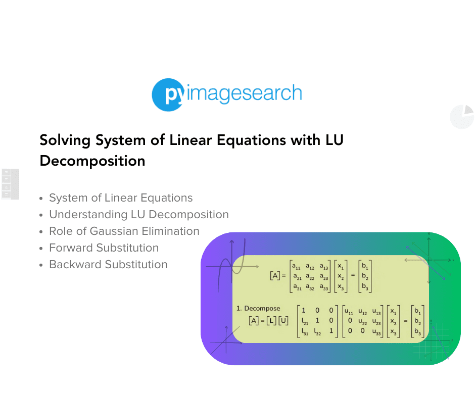
In this tutorial, you will learn how to solve a system of linear equations using the popular lower-upper (LU) decomposition.

Whether you’re working on engineering simulations, financial modeling, or scientific computing, understanding matrices and their nuances can significantly help simplify complex problems and enhance computational efficiency. One such tool is matrix factorization techniques that act as a fundamental and pivotal tool in linear algebra to represent matrices into similar components each having unique properties.

Among these techniques, LU decomposition stands out as a powerful method for solving systems of linear equations. LU decomposition leverages the fundamental principles of Gaussian elimination to break down a matrix into two easier-to-handle matrices: a lower triangular matrix and an upper triangular matrix .

This approach not only simplifies the process of solving linear systems but also provides insights into the structural properties of the matrix. In this blog post, we will delve into the intricacies of LU decomposition, explore its connection with Gaussian elimination, and guide you through practical steps to apply this method to solve linear equations effectively. By mastering LU decomposition, you’ll gain a valuable toolset for tackling a wide range of mathematical and real-world problems with confidence.

This lesson is the 1st of a 3-part series on Matrix Factorization:

1. Solving System of Linear Equations with LU Decomposition (this tutorial)
2. Diagonalize Matrix for Data Compression with Singular Value Decomposition
3. Solving System of Linear Equations with QR Decomposition

To learn how to solve a system of linear equations using popular LU decomposition, just keep reading.

---

System of Linear Equations

Picture yourself in the middle of a busy city, where everything is connected and interacting in a web of relationships. This is similar to the world of linear equations. These equations form a network of connections that explain many scientific, engineering, and economic situations.

Systems of linear equations break down complex problems into simple, manageable parts, making them essential for solving real-world issues. They turn complicated scenarios into clear mathematical expressions that we can work with, helping us understand and solve a wide range of problems.

The importance of systems of linear equations cannot be overstated. They are ubiquitous in both theoretical and applied mathematics, serving as the foundation for many disciplines:

• Engineering: Engineers use them to model and solve problems in circuits, structures, fluid dynamics, and more. Whether it’s determining the stress on a bridge or the flow rate in a pipeline, systems of linear equations provide the necessary framework.
• Economics: Economists apply them to optimize resources, forecast trends, and analyze market behaviors. They help in determining the equilibrium points in supply-demand models.
• Computer Science: Algorithms for graphics rendering, machine learning, and data analysis often rely on solving large systems of linear equations efficiently.

---

What Are Systems of Linear Equations?

At their core, systems of linear equations (Figure 1) consist of multiple linear equations involving the same set of variables. They take the form:

Here, are coefficients, are the variables, and are the constants. These equations represent lines (in 2 dimensions), planes (in 3 dimensions), or hyperplanes (in higher dimensions), and the solutions to these systems lie at the intersections of these geometric entities.

Take, for instance, an electrical engineer working with Kirchhoff’s laws to analyze a complex electrical circuit (Figure 2). Kirchhoff’s laws state that the sum of currents entering a junction must equal the sum of currents leaving it (Kirchhoff’s Current Law), and the sum of voltage drops in a closed loop must equal the sum of voltage sources (Kirchhoff’s Voltage Law).

By applying these principles to the circuit, the engineer can derive a system of linear equations (Figure 3), where variables represent the current flowing through a resistor with resistance . The constants are the voltages in the circuit. By solving this system, the engineer can determine the current distribution throughout the circuit, ensuring the design functions correctly and efficiently.

---

The Role of Matrix Factorization

While solving small systems by hand or using simple algorithms is feasible, real-world problems often involve massive datasets with thousands or even millions of variables and equations. This is where matrix factorization techniques (e.g., LU decomposition) come into play. They provide powerful tools to break down complex systems into simpler, more manageable components.

Matrix factorization (Figure 4) transforms a complex matrix into a product of simpler matrices with specific properties, making it easier to:

• Solve Linear Systems: By decomposing a matrix into simpler matrices, we can use basic substitution methods to find the solution efficiently.
• Analyze Structural Properties: Understanding the factorized components helps in gaining insights into the matrix’s properties (e.g., rank and determinant), which are crucial for stability and sensitivity analyses.
• Enhance Computational Efficiency: Factorization algorithms reduce computational complexity, making it possible to handle large-scale problems that would otherwise be intractable.

---

Understanding LU Decomposition

LU decomposition (Figure 5) is a method of expressing a matrix as the product of two simpler matrices: a lower triangular matrix and an upper triangular matrix . This factorization is useful because it simplifies many matrix operations (e.g., solving systems of linear equations, inverting matrices, and computing determinants). Here’s a detailed look at how LU decomposition works:

1. Lower Triangular Matrix (L): This matrix has zeros above the main diagonal. The entries on the diagonal are typically set to 1. This structure makes it easier to solve equations involving because each equation can be solved sequentially, starting from the first row and moving downward.
2. Upper Triangular Matrix (U): This matrix has zeros below the main diagonal. The entries on the diagonal and above are the result of the Gaussian elimination process. The upper triangular structure simplifies backward substitution, allowing us to solve equations starting from the last row and moving upward.

By decomposing into and , we transform the problem of solving into two easier problems (Figure 6):

• First, solve for using the forward substitution.
• Then, solve for using the backward substitution.

---

The Role of Gaussian Elimination

Gaussian elimination (Figure 7) is a process used to transform a matrix into an upper triangular form, which is a key step in the LU decomposition. Here’s a more detailed breakdown of how the Gaussian elimination contributes to this process:

1. Forward Elimination

• The goal of forward elimination (Figure 8) is to zero out the entries below the main diagonal of the matrix , turning it into an upper triangular matrix .
• This is achieved by using row operations. For each pivot element , we subtract a multiple of the th row from the rows below it to create zeros in the th column.
• The multipliers used in these row operations are recorded and used to construct the lower triangular matrix

2. Construction of L and U

• During the forward elimination process, the coefficients (multipliers) used to eliminate the entries below the main diagonal are stored in the matrix (Figure 9). Specifically, if is the multiplier used to eliminate the entry , it becomes an entry .

• The resulting matrix after all row operations (with zeros below the diagonal) is the upper triangular matrix (Figure 10).

---

Solving Linear Equations Using LU Decomposition

In this section, we will learn to implement the LU decomposition using the Gaussian elimination process and use it for solving a system of linear equations. As an example, let’s take the following set of linear equations (Figure 11) that are derived by applying Kirchoff’s law on the electrical circuit shown in Figure 2.

---

LU Decomposition Using Gaussian Elimination

We begin with a matrix and use the Gaussian elimination process to find the LU decomposition.

 import numpy as np

def lu_decomposition(A):
    n = len(A)
    L = np.eye(n) # initializing L as identity
    U = A.copy() # initializing U from original matrix A
   
    for i in range(n):
        for j in range(i+1, n):
            factor = U[j][i] / U[i][i] # forward elimination factor
            L[j][i] = factor # updating L matrix
            U[j, i:] -= factor * U[i, i:] # updating U matrix
   
    return L, U

# Example matrix
A = np.array([[10.0, -6.0, 0.0],
              [-6.0, 10.0, -3.0],
              [0.0, -3.0, 5.0]])

b = np.array([15.0, 0.0, -10.0])

L, U = lu_decomposition(A)
print("Matrix L : \n", L)
print("Matrix U: \n", U)
print("Verifying LU : \n", np.dot(L, U))

On Line 1, we import numpy for matrix operations. On Line 3, the lu_decomposition function is defined. On Lines 5 and 6, L is initialized as an identity matrix and U as a copy of A. On Lines 8-12, nested loops perform forward elimination to fill in L and update U. The function returns L and U on Line 14.

On Lines 17-19, we define matrix A. On Line 23, the LU decomposition is performed, and the results are printed on Lines 24 and 25. On Line 26, we verify that L and U multiply to recover A.

Output:

Matrix L : 
 [[ 1.       0.       0.     ]
 [-0.6      1.       0.     ]
 [ 0.      -0.46875  1.     ]]
Matrix U: 
 [[10.      -6.       0.     ]
 [ 0.       6.4     -3.     ]
 [ 0.       0.       3.59375]]
Verifying LU : 
 [[10. -6.  0.]
 [-6. 10. -3.]
 [ 0. -3.  5.]]

The output shows L with ones on the diagonal and U as an upper triangular matrix. The verification confirms the correctness of the decomposition.

---

Forward Substitution

Now, we have the LU decomposition of the matrix:

Next, we will perform the forward substitution, where we solve for such that:

and where .

 def forward_substitution(L, b):
    n = len(b)
    y = np.zeros_like(b)
   
    # forward substitution to solve for each variable one by one
    for i in range(n):
        y[i] = b[i] - np.dot(L[i, :i], y[:i])
   
    return y

y = forward_substitution(L, b)
print("y = Ux obtained from forward elimination : ", y)

In the forward_substitution function, we solve the lower triangular system . On Lines 27 and 28, we define the function and initialize the length of b. On Line 29, we create a zero vector y of the same length as b.

On Lines 32 and 33, we iterate through each variable, solving for y[i] by subtracting the dot product of the known elements of L and y from b[i]. The function returns the solution vector y on Line 35.

We then call this function to get y and print the result on Lines 37 and 38.

Output:

y = Ux obtained from forward elimination :  [15.       9.      -5.78125]

The output shows the intermediate solution vector y = [15.0, 9.0, -5.78125], which is essential for the next steps in solving the system of equations.

---

Backward Substitution

After solving for , we will solve for using backward substitution:

def backward_substitution(U, y):
    n = len(y)
    x = np.zeros_like(b)
   
    # forward substitution to solve for each variable one by one
    for i in range(n-1, -1, -1):
        x[i] = (y[i] - np.dot(U[i, i+1:], x[i+1:]))/U[i, i]
   
    return x

x = backward_substitution(U, y)
print("x obtained from backward elimination : ", x)

In the backward_substitution function, we solve the upper triangular system . On Lines 39 and 40, we define the function and initialize the length of y. On Line 41, we create a zero vector x of the same length as b.

On Lines 44 and 45, we iterate through each variable in reverse order, solving for x[i] by subtracting the dot product of the known elements of U and x from y[i], then dividing by the diagonal element U[i, i]. The function returns the solution vector x on Line 47.

We then call this function to get x and print the result on Lines 49 and 50.

Output:

x obtained from backward elimination :  [ 1.89130435  0.65217391 -1.60869565]

The output shows the solution vector x = [1.89130435, 0.65217391, -1.60869565], which completes the process of solving the system of equations.

---

---

Summary

In our exploration of systems of linear equations, we begin by understanding their fundamental role in translating complex real-world problems into manageable mathematical expressions. Systems of linear equations consist of multiple linear equations involving the same set of variables, forming a network of relationships that appear in various scientific, engineering, and economic contexts. This foundational understanding sets the stage for us to delve deeper into the methods used to solve these equations efficiently.

We then transition to the importance of matrix factorization, which simplifies the process of solving large and complex systems. By breaking down a matrix into simpler components, we can more easily analyze and manipulate the system. One of the key techniques in matrix factorization is LU decomposition, which involves decomposing a matrix into a lower triangular matrix (L) and an upper triangular matrix (U). Understanding this process, particularly through the lens of Gaussian Elimination, enhances our ability to solve linear systems accurately and efficiently.

To solve linear equations using LU decomposition, we employ two essential steps: forward substitution and backward substitution. Forward substitution allows us to solve for intermediate variables by iterating through the lower triangular matrix (L) and the given vector b. Backward substitution then takes these intermediate solutions and solves for the final variables by iterating through the upper triangular matrix U. By mastering these techniques, we can confidently approach and solve complex linear systems, leveraging the power of matrix factorization to enhance our problem-solving toolkit.

---

Citation Information

Mangla, P. “Solving System of Linear Equations with LU Decomposition,” PyImageSearch, P. Chugh, S. Huot, and P. Thakur, eds., 2025, https://pyimg.co/tu910

@incollection{Mangla_2025_solving-system-linear-equations-lu-decomposition,
  author = {Puneet Mangla},
  title = {{Solving System of Linear Equations with LU Decomposition}},
  booktitle = {PyImageSearch},
  editor = {Puneet Chugh and Susan Huot and Piyush Thakur},
  year = {2025},
  url = {https://pyimg.co/tu910},
}

---