Table of Contents
- Comparison Between BagofWords and Word2Vec
- A Brief Recap of BOW and Word2Vec
- Configuring Your Development Environment
- Having Problems Configuring Your Development Environment?
- Project Structure
- Configuring the Prerequisites
- Processing the Data
- Creating the Bag-of-Words Model
- Training the Bag-of-Words Model
- Training the Word2Vec Model
- Training Results and Visualizations
- Summary
Comparison Between BagofWords and Word2Vec
In the past few weeks, we have gone over important Natural Language Processing (NLP) techniques like Bag-of-Words and Word2Vec. Both are, in some form, part of representation learning in NLP.
In general, the representation of features in a way that makes the computer understand text has really helped NLP grow. But both of the techniques mentioned above are drastically different from each other. This begs the question, what makes us choose one over the other?
In this tutorial, you will go through a comparison between Bag-of-Words and Word2Vec.
This lesson is the last in a 4-part series on NLP 101:
- Introduction to Natural Language Processing (NLP)
- Introduction to the Bag-of-Words (BoW) Model
- Word2Vec: A Study of Embeddings in NLP
- Comparison Between BagofWords and Word2Vec (today’s tutorial)
To learn the difference between Bag-of-Words and Word2Vec, just keep reading.
Comparison Between BagofWords and Word2Vec
Let’s go through a brief recap of what representation learning in NLP is. Teaching text data to computers is extremely difficult and complex. In our first blog post in this series, we went over a brief history of Natural Language Processing.
There, we established how the introduction of statistics and representation learning in NLP changed the general progress of NLP in a more positive direction. We learned about Bag-of-Words (BOW), a technique that has its roots in representational learning. This was followed by a more complex and comprehensive approach of Word2Vec.
Both of these techniques involve expressing our input data into a representational (embedding) space. The more associations we can spot, the more validation we get about how well our model has learned.
Let’s take it up a notch and dig even deeper into why these techniques are similar yet drastically different.
A Brief Recap of BOW and Word2Vec
The Bag-of-Words architecture involved converting each input sentence into a bag of words. Take a look at Figure 1.

The embedding matrix here has a number of columns equal to the number of words in the total vocabulary. Each sentence is expressed as a combination of each word either appearing or not appearing.
For example, if the vocabulary size of a given dataset was 300, an input sentence of size 5 would now become a vector of size 300, with the bits of the 5 occurring words turned on while having the 295 bits turned off.
Word2Vec takes a different approach in making use of vectors. Here, instead of each sentence being represented as entities, we consider each word. We choose a finite dimensional embedding space, where each row represents a word in the vocabulary.
Throughout training, each word has some value (or weight) that it develops for each dimension, representing its vectorial form. These weights are determined by each word’s context (i.e., the neighboring words).
Hence, the sentences “The sky is blue.” and “Blue skies are beautiful.” would mean the word blue will be associated with the sky in our embedding space.
Both of these approaches are ingenious and are great in their own way. But let’s scrutinize each algorithm further.
Configuring Your Development Environment
To follow this guide, you need to have the OpenCV library installed on your system.
Luckily, OpenCV is pip-installable:
$ pip install opencv-contrib-python
If you need help configuring your development environment for OpenCV, we highly recommend that you read our pip install OpenCV guide — it will have you up and running in a matter of minutes.
Having Problems Configuring Your Development Environment?
All that said, are you:
- Short on time?
- Learning on your employer’s administratively locked system?
- Wanting to skip the hassle of fighting with the command line, package managers, and virtual environments?
- Ready to run the code right now on your Windows, macOS, or Linux system?
Then join PyImageSearch University today!
Gain access to Jupyter Notebooks for this tutorial and other PyImageSearch guides pre-configured to run on Google Colab’s ecosystem right in your web browser! No installation required.
And best of all, these Jupyter Notebooks will run on Windows, macOS, and Linux!
Project Structure
We first need to review our project directory structure.
Start by accessing the “Downloads” section of this tutorial to retrieve the source code and example images.
From there, take a look at the directory structure:
!tree .
.
├── datadf.csv
├── LICENSE
├── outputs
│   ├── loss_BOW.png
│   ├── loss_W2V.png
│   ├── terminal_outputs.txt
│   ├── TSNE_BOW.png
│   └── TSNE_W2V.png
├── pyimagesearch
│   ├── BOWmodel.py
│   ├── config.py
│   ├── data_processing.py
│   └── __init__.py
├── README.md
├── train_BOW.py
└── train_Word2Vec.py

2 directories, 14 files
We have two sub-directories: outputs and pyimagesearch.
Inside the outputs directory, we have all the results and visualizations of this project.
In the pyimagesearch directory, we have:
BOWmodel.py: Contains the model architecture for Bag-of-Words.config.py: Contains the entire configuration pipeline.data_processing.py: A script that houses several data processing utilities.__init__.py: Makes thepyimagesearchdirectory act like a python package.
In the main directory, we have:
train_BOW.py: Training script for Bag-of-Words architecture.train_Word2Vec.py: Training script for Word2Vec architecture.datadf.csv: The training data for our project.
Configuring the Prerequisites
Inside the pyimagesearch directory, the config.py script houses the entire configuration pipeline for our project.
# import the necessary packages
import os

# define Bag-of-Words parameters
EPOCHS = 30

# define the Word2Vec parameters
EMBEDDING_SIZE = 2
ITERATIONS = 1000

# define the path to the output directory
OUTPUT_PATH = "outputs"

# define the path to the Bag-of-Words output
BOW_LOSS = os.path.join(OUTPUT_PATH, "loss_BOW")
BOW_TSNE = os.path.join(OUTPUT_PATH, "TSNE_BOW")

# define the path to the Word2vec output
W2V_LOSS = os.path.join(OUTPUT_PATH, "loss_W2V")
W2V_TSNE = os.path.join(OUTPUT_PATH, "TSNE_W2V")
On Line 5, we define the number of epochs where the bag-of-words model will be trained.
On Lines 8 and 9, we define parameters for the Word2Vec model, namely the number of embedding dimensions and iterations for which the Word2Vec model will train.
Next, the outputs directory is defined (Line 12), followed by individual definitions for the loss and TSNE plots (Lines 15-20).
Processing the Data
We will be moving on to the data processing script data_processing.py. This script houses functions to help us with managing the data.
# import the necessary packages
import re
import tensorflow as tf

def preprocess(sentDf, stopWords, key="sentence"):
	# loop over all the sentences
	for num in range(len(sentDf[key])):
		# strip the sentences off the stop-words
		newSent = ""
		for word in sentDf["sentence"].iloc[num].split():
			if word not in stopWords:
				newSent = newSent + " " + word

	# update the sentences
	sentDf["sentence"].iloc[num] = newSent

	# return the preprocessed data
	return(sentDf)
On Line 5, we have the first function, preprocess, which takes in the following arguments:
sentDf: The input dataframe.stopWords: A list of words to omit from our dataset.key: Set tosentenceby default. It will be used to access the right column of the dataframe.
Looping over the sentences on Line 7, we first initialize an empty string to store our processed data on Line 9. Now, each word in the sentence is iterated through (Line 10), and the stopwords are omitted.
We update the dataframe with the new sentences (without the stop-words) on Line 15.
def prepare_tokenizerBOW(df, topWords, sentKey="sentence", outputKey="sentiment"):
	# prepare separate tokenizers for the data and labels
	tokenizerData = tf.keras.preprocessing.text.Tokenizer(num_words=topWords,
			oov_token="<unk>",
			filters='!"#$%&()*+.,-/:;=?@[\]^_`{|}~')
	tokenizerLabels = tf.keras.preprocessing.text.Tokenizer(num_words=5,
			oov_token="<unk>",
			filters='!"#$%&()*+.,-/:;=?@[\]^_`{|}~')

	# fit the tokenizers on their respective data
	tokenizerData.fit_on_texts(df["sentence"])
	tokenizerLabels.fit_on_texts(df["sentiment"])

	# return the tokenizers
	return (tokenizerData, tokenizerLabels)
Our next function is prepare_tokenizerBOW on Line 20, which takes in the following arguments:
df: The input dataframe stripped off the stop-words.topWords: An argument required to initialize the tensorflow tokenizer.sentKey: The key to access the sentences from the dataframe.outputKey: The key to access the labels from the dataframe.
This function is specifically for the Bag-of-Words architecture, where we will be using two separate tokenizers for the data and their labels. Accordingly, we create the two tokenizers and fit them on their respective texts (Lines 22-31).
def prepare_tokenizerW2V(df, topWords, sentKey="sentence", outputKey="sentiment"):
	# prepare tokenizer for the Word2Vec data
	tokenizerWord2Vec = tf.keras.preprocessing.text.Tokenizer(num_words=topWords,
			oov_token="<unk>",
			filters='!"#$%&()*+.,-/:;=?@[\]^_`{|}~')

	# fit the tokenizer on the data
	tokenizerWord2Vec.fit_on_texts(df["sentence"])
	tokenizerWord2Vec.fit_on_texts(df["sentiment"])

	# return the tokenizer
	return (tokenizerWord2Vec)
The final function in this script is the prepare_tokenizerW2V on Line 36, which takes in the following arguments:
df: The input dataframe stripped off the stop-words.topWords: An argument required to initialize the tensorflow tokenizer.sentKey: The key to access the sentences from the dataframe.outputKey: The key to access the labels from the dataframe.
On Lines 38-40, we have initialized a single tokenizer for the Word2Vec approach and fit it on the data and labels on Lines 43 and 44. Since both approaches are different, we are using a single tokenizer.
Creating the Bag-of-Words Model
Next, we will define the architecture of the Bag-of-Words model. Let’s move into the BOWmodel.py script.
#import the necessary packages
import tensorflow as tf
from tensorflow.keras.layers import Dense
from tensorflow.keras.models import Sequential
from tensorflow.keras.losses import sparse_categorical_crossentropy

def build_shallow_net(inputDims, numClasses):
	# define the model
	model = Sequential()
	model.add(Dense(512, input_dim=inputDims, activation="relu"))
	model.add(Dense(128, activation="relu"))
	model.add(Dense(numClasses, activation="softmax"))

	# compile the keras model
	model.compile(loss=sparse_categorical_crossentropy,
			optimizer="adam",
			metrics=["accuracy"]
	)

	# return model
	return model
On Line 7, we have build_shallow_Net, which takes in the following arguments:
inputDims: The input dimension equal to the number of words in the vocabulary.numClasses: The number of output classes.
On Lines 9-12, we define a sequential model consisting of two dense layers and a final softmax dense layer. Since we are dealing with small data, a simple model like this will work fine.
On Lines 15-18, we compile the model with sparse_categorical_crossentropy loss and adam optimizer, with accuracy as our metric.
Training the Bag-of-Words Model
To train the Bag-of-Words architecture, we will move into the train_BOW.py script.
# USAGE
# python -W ignore train_BOW.py

# set seed for reproducibility
import tensorflow as tf
tf.random.set_seed(42)

# import the necessary packages
from pyimagesearch import config
from pyimagesearch.data_processing import preprocess
from pyimagesearch.BOWmodel import build_shallow_net
from pyimagesearch.data_processing import prepare_tokenizerBOW
from sklearn.manifold import TSNE
import matplotlib.pyplot as plt
from tqdm import tqdm
import pandas as pd
import numpy as np
import nltk
import os

# prepare stop-words using the NLTK package
nltk.download("stopwords")
stopWords = nltk.corpus.stopwords.words("english")

# initialize the dataframe from csv format
dataDf = pd.read_csv("datadf.csv")

# preprocess the dataframe
processedDf = preprocess(dataDf, stopWords)
The first step in this script is to create the stopWords list. For this, we will be taking the help of the nltk package (Lines 22 and 23). Next, we initialize the dataframe using the input file in csv format (Line 26). This is followed by using the preprocess function to remove the stop-words from the input sentences (Line 29).
# store the number of classification heads
numClasses = len(processedDf["sentiment"].unique())

# create the tokenizers for data and labels
(tokenizerData, tokenizerLabels) = prepare_tokenizerBOW(processedDf, topWords=106)

# create integer sequences of the data using tokenizer
trainSeqs = tokenizerData.texts_to_sequences(processedDf["sentence"])
trainLabels = tokenizerLabels.texts_to_sequences(processedDf["sentiment"])

# create the Bag-of-Words feature representation
encodedDocs = tokenizerData.texts_to_matrix(processedDf["sentence"].values,
		mode="count"
)

# adjust the train label indices for training
trainLabels = np.array(trainLabels)
for num in range(len(trainLabels)):
	trainLabels[num] = trainLabels[num] - 1

# initialize the model for training
BOWModel = build_shallow_net(inputDims = tokenizerData.num_words-1,
		numClasses=numClasses
)

# fit the data into the model and store training details
history = BOWModel.fit(encodedDocs[:, 1:],
		trainLabels.astype('float32'),
		epochs=config.EPOCHS
)
On Line 32, the number of output classes is stored. Next, the tokenizers for the data and labels are obtained using the prepare_tokenizerBOW function on Line 35.
Now we can convert our words into integer sequences using the texts_to_sequences function on Lines 38 and 39.
Using the texts_to_matrix function, we convert our input text into the Bag-of-Words representation by setting the mode argument to count (Lines 42-44). This will count the number of times a word has occurred in a sentence, giving us vectorial representations of the sentences and occurrences for each word.
On Lines 47-49, we adjust the indices of the labels for training. The Bag-of-Words model is initialized (Lines 52-54), and the model is trained on the input data accordingly (Lines 57-60). Since the tokenizer creation adds the unknown word token as its first entry, we have considered all the words except starting from the 1st index and not the 0th index.
# create output directory if it doesn't already exist
if not os.path.exists(config.OUTPUT_PATH):
	os.makedirs(config.OUTPUT_PATH)

# plot the loss for BOW model
print("[INFO] Plotting loss...")
plt.plot(history.history["loss"])
plt.xlabel("epoch")
plt.ylabel("loss")
plt.savefig(config.BOW_LOSS)

# get the weights for the first model layer
representationsBOW = BOWModel.get_weights()[0]

# apply dimensional reduction using TSNE
tsneEmbed = (TSNE(n_components=2)
		.fit_transform(representationsBOW)
)

# initialize a index counter
indexCount = 1

# initialize the tsne figure
plt.figure(figsize=(25, 5))

# loop over the tsne embeddings and plot the corresponding words
print("[INFO] Plotting TSNE embeddings...")
for (word, embedding) in tsneEmbed[:100]:
	plt.scatter(word, embedding)
	plt.annotate(tokenizerData.index_word[indexCount], (word, embedding))
	indexCount += 1
plt.savefig(config.BOW_TSNE)
On Lines 63 and 64, we create the outputs folder if it doesn’t exist already.
On Lines 67-71, we plot the model loss with the help of the model history variable.
Now, we want to plot the Bag-of-Words representation space. Notice how the first layer of the model has the input dimensions equal to the number of words. If we assume each column corresponds to each word in the dataset, the weights of this layer can be considered our embedding space.
Hence, grab the weights of this layer on Line 74 and apply TSNE embedding for dimension reductions (Lines 77-79). We proceed to plot the TSNE plot for each word for inference.
Training the Word2Vec Model
Now we will move on to the Word2Vec model. To train it, we have to execute the train_Word2Vec.py.
# USAGE
# python -W ignore train_Word2Vec.py

# set seed for reproducibility
import tensorflow as tf
tf.random.set_seed(42)

# import the necessary packages
from pyimagesearch import config
from pyimagesearch.data_processing import preprocess
from pyimagesearch.data_processing import prepare_tokenizerW2V
from sklearn.manifold import TSNE
import matplotlib.pyplot as plt
import tensorflow as tf
from tqdm import tqdm
import pandas as pd
import numpy as np
import nltk
import os

# prepare stop-words using the NLTK package
nltk.download("stopwords")
stopWords = nltk.corpus.stopwords.words("english")

# initialize the dataframe from csv format
dataDf = pd.read_csv("datadf.csv")

# preprocess the dataframe
processedDf = preprocess(dataDf, stopWords)
As done in the Bag-of-Words script, the first step in this script is to create the stopWords list. For this, we will be taking the help of the nltk package (Lines 22 and 23). Next, we initialize the dataframe using the input file in csv format (Line 26). This is followed by using the preprocess function to remove the stop-words from the input sentences (Line 29).
# store the number of classification heads
numClasses = len(processedDf["sentiment"].unique())

# create the tokenizers for data and labels
(tokenizerData) = prepare_tokenizerW2V(processedDf, topWords=200)

# create integer sequences of the data using tokenizer
trainSeqs = tokenizerData.texts_to_sequences(processedDf["sentence"])
trainLabels = tokenizerData.texts_to_sequences(processedDf["sentiment"])

# create the representational matrices as variable tensors
contextVectorMatrix =  tf.Variable(
	np.random.rand(200, config.EMBEDDING_SIZE)
)
centerVectorMatrix = tf.Variable(
	np.random.rand(200, config.EMBEDDING_SIZE)
)

# initialize the optimizer and create an empty list to log the loss
optimizer = tf.optimizers.Adam()
lossList = list()
On Line 32, we store the number of output classes. Next, the single tokenizer covering both the data and labels is created on Line 35.
The word sequences are converted into integer sequences using the texts_to_sequences function of the tokenizer (Lines 38 and 39).
For the Word2Vec architecture, we then initialize the context and center word matrices on Lines 42-47. This is followed by the Adam optimizer and an empty loss-list initialization (Lines 50 and 51).
# loop over the training epochs
print("[INFO] Starting Word2Vec training...")
for iter in tqdm(range(config.ITERATIONS)):
	# initialize the loss per epoch
	lossPerEpoch = 0

	# loop over the indexes and labels
	for idxs,trgt in zip(trainSeqs, trainLabels):
		# convert label into integer
		trgt = trgt[0]

		# initialize the gradient tape
		with tf.GradientTape() as tape:
			# initialize the combined context vector
			combinedContext = 0

			# update the combined context with each index
			for count,index in enumerate(idxs):
				combinedContext += contextVectorMatrix[index,:]

			# standardize the vector
			combinedContext /= len(idxs)

			# matrix multiply the center vector matrix
			# with the combined context
			output = tf.matmul(centerVectorMatrix,
				tf.expand_dims(combinedContext ,1))

			# calculate the softmax output and
			# grab the relevant index for loss calculation
			softOut = tf.nn.softmax(output, axis=0)
			loss = softOut[trgt]
			logLoss = -tf.math.log(loss)

		# update the loss per epoch and apply the gradients to the
		# embedding matrices
		lossPerEpoch += logLoss.numpy()
		grad = tape.gradient(
			logLoss, [contextVectorMatrix, centerVectorMatrix]
		)
		optimizer.apply_gradients(
			zip(grad, [contextVectorMatrix, centerVectorMatrix])
		)

	# update the loss list
	lossList.append(lossPerEpoch)
On Line 55, we start iterating over the training epochs and initialize a lossPerEpoch variable on Line 57.
Next, we loop over the indices and labels of the training sequence and labels (Line 60) and first convert the label list into a single variable (Line 62).
We initialize a gradient tape on Line 65. The sentence indices are used to extract the context vectors from the context matrix, and the outputs are added together, followed by normalization (Lines 67-74).
The combined context vector is multiplied by the center vector matrix, and the result is passed through a softmax function (Lines 78-83). The relevant center word index is grabbed for loss calculation, and the negative logarithm of the index is calculated (Lines 84 and 85).
Once out of the loop, the lossPerEpoch variable is updated. The gradients are applied to the two embedding matrices (Lines 89-95).
Finally, once an epoch is over, the lossPerEpoch variable is added to the loss list (Line 98).
# create output directory if it doesn't already exist
if not os.path.exists(config.OUTPUT_PATH):
	os.makedirs(config.OUTPUT_PATH)

# plot the loss for evaluation
print("[INFO] Plotting Loss...")
plt.plot(lossList)
plt.xlabel("epoch")
plt.ylabel("loss")
plt.savefig(config.W2V_LOSS)

# apply dimensional reductionality using tsne for the
# representation matrices
tsneEmbed = (
	TSNE(n_components=2)
	.fit_transform(contextVectorMatrix.numpy())
)

# initialize a index counter
indexCount = 1

# initialize the tsne figure
plt.figure(figsize=(25, 5))

# loop over the tsne embeddings and plot the corresponding words
print("[INFO] Plotting TSNE Embeddings...")
for (word, embedding) in tsneEmbed[:100]:
	if indexCount != 108:
		plt.scatter(word, embedding)
		plt.annotate(tokenizerData.index_word[indexCount], (word, embedding))
		indexCount += 1
plt.savefig(config.W2V_TSNE)
On Lines 101 and 102, we create the outputs folder if it doesn’t exist already.
On Lines 105-109, we plot the loss for the Word2Vec model. This is followed by creating the TSNE plot from the embedding matrix (Lines 113-131). The words corresponding to their indices are plotted on the TSNE plot to assess associations formed.
Training Results and Visualizations
Let’s look at how the training for both the architectures fared.
[nltk_data] Downloading package stopwords to /root/nltk_data...
[nltk_data]   Package stopwords is already up-to-date!
Epoch 1/30
1/1 [==============================] - 0s 452ms/step - loss: 1.4033 - accuracy: 0.2333
Epoch 2/30
1/1 [==============================] - 0s 4ms/step - loss: 1.2637 - accuracy: 0.7000
Epoch 3/30
1/1 [==============================] - 0s 4ms/step - loss: 1.1494 - accuracy: 0.8667
...
Epoch 27/30
1/1 [==============================] - 0s 5ms/step - loss: 0.0439 - accuracy: 1.0000
Epoch 28/30
1/1 [==============================] - 0s 4ms/step - loss: 0.0374 - accuracy: 1.0000
Epoch 29/30
1/1 [==============================] - 0s 3ms/step - loss: 0.0320 - accuracy: 1.0000
Epoch 30/30
1/1 [==============================] - 0s 3ms/step - loss: 0.0275 - accuracy: 1.0000
[INFO] Plotting loss...
[INFO] Plotting TSNE embeddings...
With our small input dataset, the Bag-of-Words model quickly reached 100% accuracy and fit on the data. However, we will leave our final assessment based on the TSNE plots. The Loss plot can be seen in Figure 3.
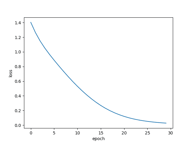
The loss dipped pretty nicely. For the given dataset, our model overfits on it perfectly.
[nltk_data] Downloading package stopwords to /root/nltk_data...
[nltk_data]   Package stopwords is already up-to-date!
[INFO] Starting Word2Vec training...
100% 1000/1000 [04:52<00:00,  3.42it/s]
[INFO] Plotting Loss...
[INFO] Plotting TSNE Embeddings...
Since the Word2Vec model is built directly by us, we will be assessing the loss based on the loss plot in Figure 4.
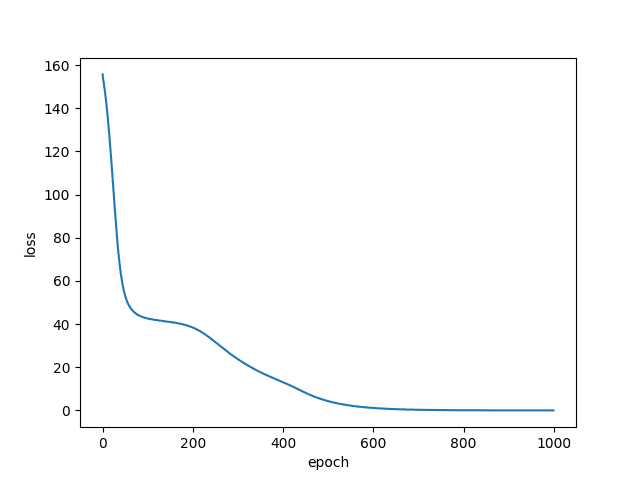
The Word2Vec loss, albeit more difficult than the Bag-of-Words (since there are more labels), dipped nicely for our small dataset. Let’s look at the TSNE plots!
In Figures 5 and 6, we have the TSNE plots for Bag-of-Words and Word2Vec, respectively.
Upon closer inspection (click to enlarge the image), we can see that although no definite groupings have formed, there are some similar context words in more or less close proximity to each other. For example, we can see food items like “burger” and “pizza” close to each other.
However, we must remember that in Bag-of-Words, complete sentences are considered as inputs. This can be why no definite groupings are formed for words. Another reason can be that dimensional reductionality has led to a loss of information. Adding another dense layer makes it less dependent on the weights of the layer we are considering.
In Figure 6, we have the TSNE plot for Word2Vec.
Instantly, we can see that several groupings are seen. You can zoom in to these images in the colaboratory version of the code and check the groupings. The difference between standard Continuous Bag-of-Words and what we have done today lies in the fact that rather than considering windows and center words in sentences, we have a definite label for each sentence.
This has made it easier for the matrices to create groupings upon training. The result here is clearly better than Bag-of-Words. However, if you want to draw your own conclusions, don’t forget to try this on your own data.
What's next? We recommend PyImageSearch University.
86+ total classes • 115+ hours hours of on-demand code walkthrough videos • Last updated: April 2026
★★★★★ 4.84 (128 Ratings) • 16,000+ Students Enrolled
I strongly believe that if you had the right teacher you could master computer vision and deep learning.
Do you think learning computer vision and deep learning has to be time-consuming, overwhelming, and complicated? Or has to involve complex mathematics and equations? Or requires a degree in computer science?
That’s not the case.
All you need to master computer vision and deep learning is for someone to explain things to you in simple, intuitive terms. And that’s exactly what I do. My mission is to change education and how complex Artificial Intelligence topics are taught.
If you're serious about learning computer vision, your next stop should be PyImageSearch University, the most comprehensive computer vision, deep learning, and OpenCV course online today. Here you’ll learn how to successfully and confidently apply computer vision to your work, research, and projects. Join me in computer vision mastery.
Inside PyImageSearch University you'll find:
- ✓ 86+ courses on essential computer vision, deep learning, and OpenCV topics
- ✓ 86 Certificates of Completion
- ✓ 115+ hours hours of on-demand video
- ✓ Brand new courses released regularly, ensuring you can keep up with state-of-the-art techniques
- ✓ Pre-configured Jupyter Notebooks in Google Colab
- ✓ Run all code examples in your web browser — works on Windows, macOS, and Linux (no dev environment configuration required!)
- ✓ Access to centralized code repos for all 540+ tutorials on PyImageSearch
- ✓ Easy one-click downloads for code, datasets, pre-trained models, etc.
- ✓ Access on mobile, laptop, desktop, etc.
Summary
In today’s tutorial, we learned the fundamental difference between Bag-of-Words and Word2Vec. Both are big stepping stones in the world of NLP, but it is important to understand why both of these techniques adhere to the usage of embeddings in their own way.
We worked on a small dataset to understand the essence of where these two approaches diverge. The TSNE plots show a substantial difference, even though the BOW architecture showed a lower final loss value. That leaves an intriguing conclusion about understanding more about embedding spaces.
A trip back to our 2nd blog post in this series would show us that the Word2Vec approaches had very high loss values. But despite that, the visualizations were very intuitive and showed many visual groupings. The reason for the high loss can be explained by the many “labels” based on the several center words appearing for each sentence.
However, that issue is no longer prevalent here since we have fixed labels for each sentence. So naturally, the Word2Vec approach showed instant groupings for this dataset.
This can be further experimented upon with a bigger dataset to reach more definitive conclusions. Still, the results today question the right metric to use when assessing an approach.
Citation Information
Chakraborty, D. “Comparison Between Bag-of-Words and Word2Vec,” PyImageSearch, P. Chugh, A. R. Gosthipaty, S. Huot, K. Kidriavsteva, R. Raha, and A. Thanki, eds., 2022, https://pyimg.co/txq23
@incollection{Chakraborty_2022_Comparison,
  author = {Devjyoti Chakraborty},
  title = {Comparison Between {BagofWords} and {Word2Vec}},
  booktitle = {PyImageSearch},
  editor = {Puneet Chugh and Aritra Roy Gosthipaty and Susan Huot and Kseniia Kidriavsteva and Ritwik Raha and Abhishek Thanki},
  year = {2022},
  note = {https://pyimg.co/txq23},
}
Unleash the potential of computer vision with Roboflow - Free!
- Step into the realm of the future by signing up or logging into your Roboflow account. Unlock a wealth of innovative dataset libraries and revolutionize your computer vision operations.
- Jumpstart your journey by choosing from our broad array of datasets, or benefit from PyimageSearch’s comprehensive library, crafted to cater to a wide range of requirements.
- Transfer your data to Roboflow in any of the 40+ compatible formats. Leverage cutting-edge model architectures for training, and deploy seamlessly across diverse platforms, including API, NVIDIA, browser, iOS, and beyond. Integrate our platform effortlessly with your applications or your favorite third-party tools.
- Equip yourself with the ability to train a potent computer vision model in a mere afternoon. With a few images, you can import data from any source via API, annotate images using our superior cloud-hosted tool, kickstart model training with a single click, and deploy the model via a hosted API endpoint. Tailor your process by opting for a code-centric approach, leveraging our intuitive, cloud-based UI, or combining both to fit your unique needs.
- Embark on your journey today with absolutely no credit card required. Step into the future with Roboflow.
To download the source code to this post (and be notified when future tutorials are published here on PyImageSearch), simply enter your email address in the form below!

Download the Source Code and FREE 17-page Resource Guide
Enter your email address below to get a .zip of the code and a FREE 17-page Resource Guide on Computer Vision, OpenCV, and Deep Learning. Inside you'll find my hand-picked tutorials, books, courses, and libraries to help you master CV and DL!


Comment section
Hey, Adrian Rosebrock here, author and creator of PyImageSearch. While I love hearing from readers, a couple years ago I made the tough decision to no longer offer 1:1 help over blog post comments.
At the time I was receiving 200+ emails per day and another 100+ blog post comments. I simply did not have the time to moderate and respond to them all, and the sheer volume of requests was taking a toll on me.
Instead, my goal is to do the most good for the computer vision, deep learning, and OpenCV community at large by focusing my time on authoring high-quality blog posts, tutorials, and books/courses.
If you need help learning computer vision and deep learning, I suggest you refer to my full catalog of books and courses — they have helped tens of thousands of developers, students, and researchers just like yourself learn Computer Vision, Deep Learning, and OpenCV.
Click here to browse my full catalog.