Word2Vec: A Study of Embeddings in NLP

---

Table of Contents

---

Word2Vec: A Study of Embeddings in NLP

Last week, we saw how representing text in a constrained manner with respect to the complete corpus helped a computer assign meaning to words. Our approach (Bag-of-Words) was based on the frequency of words and required complex computations when the input text got bigger. But the idea of representation that it presented was worth exploring.

We slowly step into the territory of modern-day Natural Language Processing (NLP) with today’s spotlight: Word2Vec.

In this tutorial, you will learn how to implement Word2Vec approaches for text.

As a small preface, Word2Vec was one of the most simple yet one of my favorite topics in NLP that I had encountered in my own journey. The idea was so simple, yet it redefined the NLP world in many ways. Let’s explore and understand the essence behind Word2Vec.

This lesson is the 3rd in a 4-part series on NLP 101:

1. Introduction to Natural Language Processing (NLP)
2. Introduction to the Bag-of-Words (BoW) Model
3. Word2Vec: A Study of Embeddings in NLP (today’s tutorial)
4. Comparison between BagofWords and Word2Vec

To learn how to implement Word2Vec, just keep reading.

---

Word2Vec: A Study of Embeddings in NLP

---

Introduction to Word2Vec

Let us address the very first thing; What does the name Word2vec mean?

It is exactly what you think (i.e., words as vectors). Word2Vec essentially means expressing each word in your text corpus in an N-dimensional space (embedding space). The word’s weight in each dimension of that embedding space defines it for the model.

But how will we assign these weights? It is not abundantly clear that teaching grammar and other semantics to a computer is a tough task but expressing the meaning of each word is a different ball game altogether. On top of that, the English language has several words with multiple meanings based on the context. So are these weights assigned at random (Table 1)?

	Alive	Wealth	Gender
Man	1	-1	-1
Queen	1	1	1
Box	-1	0	0
Table 1: Embeddings.

Believe it or not, the answer lies in the last paragraph itself. We help define the meaning of words based on their context.

Now, if that sounds confusing to you, let’s break it down into even simpler terms. The context of a word is defined by its neighboring words. Hence, the meaning of a word will depend on the words where it is associated.

If your text corpus has several instances of the word “read” in the same sentence as the word “book”, the Word2Vec approach will automatically group them together. Hence, this technique is totally dependent on a good dataset.

Now that we have determined the magic of Word2Vec lies in word associations, let us take it a step further and understand the two subsets of Word2Vec.

---

Continuous Bag-of-Words (CBOW)

CBOW is a technique where, given the neighboring words, the center word is determined. If our input sentence is “I am reading the book.”, then the input pairs and labels for a window size of 3 would be:

• I, reading, for the label am
• am, the, for the label reading
• reading, book, for the label the

Take a look at Figure 1.

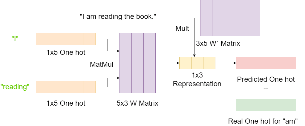
Let’s assume our input sentence in Figure 1 is our complete input text. That makes our vocabulary size 5, and we will assume there are 3 embedding dimensions for simplicity.

We will be considering the example of the input-label pair of (I, reading) – (am). We start with the one-hot encodings of I and reading (shape 1x5), multiplying those encodings with an encoding matrix of shape 5x3. The result is a 1x3 hidden layer.

This hidden layer is now multiplied by a 3x5 decoding matrix to give us our prediction of a 1x5 shape. This is compared to the actual label (am) one-hot encoding of the same shape to complete the architecture.

The star here is the encoding/decoding matrices. The loss affects the weights of these matrices in adapting to the data. The matrices provide a finite space in which each word is expressed. The matrices become the vectorial representation for the words.

A single matrix can be used to fulfill both encoding/decoding purposes. For disentanglement between these two tasks, we will be using two matrices: the context word matrix to represent the words when viewing them as the neighboring words and the center word matrix to represent the words when viewing them as the center words.

Using two matrices gives each word two different spheres of space in which they exist while giving us two different perspectives to view each word.

---

Skip-Gram

The second technique in today’s spotlight is the Skip-Gram approach. Here, given the center word, we have to predict its neighboring words. Quite literally the opposite of CBOW, but more efficient. Before we get to that, let’s understand what Skip-Gram is.

Let our given input sentence be “I am reading the book.” The corresponding Skip-Gram pairs for a window size of 3 would be:

• am, for labels I and reading
• reading, for labels am and the
• the, for labels reading and book

Let’s analyze Figure 2.

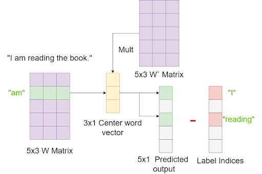
Just as in CBOW, let’s assume our input sentence in Figure 2 is our complete input text. That makes our vocabulary size 5, and we will assume there are 3 embedding dimensions for simplicity.

Starting with the encoding matrix, we grab the vector located at the index of our center word (am in this case). Transposing it, we now have a 3x1 vector representation of the word am (since we are directly grabbing a row of the encoding matrix, this WILL NOT be a one-hot encoding).

We multiply this vector representation with the decoding matrix of shape 5x3, giving us the predicted output of shape 5x1. Now, this vector will essentially be a softmax representation over the whole vocabulary, pointing to the indices belonging to the neighboring words of our input center word. In this case, the output should point to the indices of I and reading.

Again, we will work with two different matrices for better representations. Skip-Gram will intuitively work better than CBOW because we are grouping several words based on a single input word, while in CBOW, we are trying to associate one single word based on several input words.

With a basic understanding of these two techniques out of the way, let’s see how we can implement CBOW and Skip-Gram.

---

Configuring Your Development Environment

To follow this guide, you need to have the OpenCV library installed on your system.

Luckily, OpenCV is pip-installable:

$ pip install opencv-contrib-python
$ pip install tensorflow

If you need help configuring your development environment for OpenCV, we highly recommend that you read our pip install OpenCV guide — it will have you up and running in a matter of minutes.

---

Having Problems Configuring Your Development Environment?

All that said, are you:

• Short on time?
• Learning on your employer’s administratively locked system?
• Wanting to skip the hassle of fighting with the command line, package managers, and virtual environments?
• Ready to run the code right now on your Windows, macOS, or Linux system?

Then join PyImageSearch University today!

Gain access to Jupyter Notebooks for this tutorial and other PyImageSearch guides that are pre-configured to run on Google Colab’s ecosystem right in your web browser! No installation required.

And best of all, these Jupyter Notebooks will run on Windows, macOS, and Linux!

---

Project Structure

We first need to review our project directory structure.

Start by accessing the “Downloads” section of this tutorial to retrieve the source code and example images.

From there, take a look at the directory structure:

!tree .
.
├── data.txt
├── LICENSE
├── outputs
│   ├── loss_CBOW.png
│   ├── loss_skipgram.png
│   ├── output.txt
│   ├── TSNE_CBOW.png
│   └── tsne_skipgram.png
├── pyimagesearch
│   ├── config.py
│   ├── create_vocabulary.py
│   └── __init__.py
├── README.md
├── requirements.txt
├── train_CBOW.py
└── train_SkipGram.py

2 directories, 14 files

We have two sub-directories in the main directory, outputs and pyimagesearch.

The outputs directory contains all the results and visualizations of our project. The pyimagesearch directory contains several scripts:

• config.py: Contains the complete configuration pipeline.
• create_vocabulary.py: Helps create the vocabulary for our project.
• __init__.py: Makes the pyimagesearch directory work as a python package.

In the parent directory, we have:

• train_CBOW.py: Training script for CBOW architecture.
• train_SkipGram.py: Training script for Skip-Gram architecture.
• data.txt: Contains the training data for our project.

---

Configuring the Prerequisites

Inside the pyimagesearch directory, the config.py script houses the configuration pipeline for our project.

# import the necessary packages
import os

# define the number of embedding dimensions
EMBEDDING_SIZE = 10

# define the window size and number of iterations
WINDOW_SIZE = 5
ITERATIONS = 1000

# define the path to the output directory
OUTPUT_PATH = "outputs"

# define the path to the skipgram outputs
SKIPGRAM_LOSS = os.path.join(OUTPUT_PATH, "loss_skipgram")
SKIPGRAM_TSNE = os.path.join(OUTPUT_PATH, "tsne_skipgram")

# define the path to the CBOW outputs
CBOW_LOSS = os.path.join(OUTPUT_PATH, "loss_cbow")
CBOW_TSNE = os.path.join(OUTPUT_PATH, "tsne_cbow")

On Line 5, we have defined the number of dimensions for your embedding matrices. Next, we define the window size for our context words and the number of iterations (Lines 8 and 9).

The output path is defined on Line 12, followed by the loss and TSNE plots for the Skip-Gram architecture. We do the same for the CBOW loss and TSNE plots (Lines 19 and 20).

---

Building the Vocabulary

In our parent directory, we have a file called data.txt, which houses the text we will use to showcase the Word2Vec techniques. In this case, we are using a paragraph about Nobel Prize laureate Marie Curie.

However, to apply the Word2Vec algorithms, we need to process the data correctly. That involves tokenization. The create_vocabulary.py script inside the pyimagesearch directory will help us build the vocabulary for our project.

# import the necessary packages
import tensorflow as tf

def tokenize_data(data):
  # convert the data into tokens
  tokenizedText = tf.keras.preprocessing.text.text_to_word_sequence(
    input_text=data
  )
  
  # create and store the vocabulary of unique words along with the
  # size of the tokenized texts
  vocab = sorted(set(tokenizedText))
  tokenizedTextSize = len(tokenizedText)

  # return the vocabulary, size of the tokenized text, and the 
  # tokenized text
  return (vocab, tokenizedTextSize, tokenizedText) 

On Line 4, we have a function called tokenize_data, which takes the text data as its argument. Thankfully, due to tensorflow, we can directly tokenize our data using tf.keras.preprocessing.text.text_to_word_sequence. This confirms all the words inside our text data into tokens.

Now, if we sort the tokenized text, this will give us the vocabulary (Line 12). This is because the tokens are created based on paradigms like alphabetical order. So our initial tokenizedText variable only has the tokenized version of the text, not the sorted vocabulary.

On Line 17, we return the created vocabulary, the size of the tokenized text, and the tokenized text itself.

---

Training the CBOW Architecture

We will start with the CBOW implementation. In the parent directory, the train_CBOW.py script houses the complete CBOW implementation.

# USAGE
# python -W ignore train_CBOW.py

# set seed for reproducibility
import tensorflow as tf
tf.random.set_seed(42)

# import the necessary packages
from pyimagesearch import config
from pyimagesearch.create_vocabulary import tokenize_data
from sklearn.manifold import TSNE
import matplotlib.pyplot as plt
from tqdm import tqdm
import pandas as pd
import numpy as np
import os

# read the text data from the disk
print("[INFO] reading the data from the disk...")
with open("data.txt") as filePointer:
  lines = filePointer.readlines()
textData = "".join(lines)

To start, we will first grab the data and convert it into a format suitable for our create_vocabulary script. On Lines 20-22, we open the data.txt file and read the lines inside it. However, this will yield a list that contains all the lines in individual string format.

To tackle that, we simply use the "".join function and join all the lines into one string.

# tokenize the text data and store the vocabulary, the size of the
# tokenized text, and the tokenized text
(vocab, tokenizedTextSize, tokenizedText) = tokenize_data(
  data=textData
)

# map the vocab words to individual indices and map the indices to
# the words in vocab
vocabToIndex = {
  uniqueWord:index for (index, uniqueWord) in enumerate(vocab)
}
indexToVocab = np.array(vocab)

# convert the tokens into numbers
textAsInt = np.array([vocabToIndex[word] for word in tokenizedText])

# create the representational matrices as variable tensors
contextVectorMatrix =  tf.Variable(
  np.random.rand(tokenizedTextSize, config.EMBEDDING_SIZE)
)
centerVectorMatrix = tf.Variable(
  np.random.rand(tokenizedTextSize, config.EMBEDDING_SIZE)
)

With our data in the correct format, we can now tokenize the data using the tokenize_data function on Lines 26-28.

Using the built vocabulary, we can map the words to their indices and create a vocabToIndex dictionary, helping us link the words to their indices (Lines 32-34).

Similarly, we create an indexToVocab variable on Line 35. The final step here is to convert our entire text data from word format to indices format on Line 38.

Now, it’s time to create our embedding spaces. As mentioned earlier, we will be using two different matrices, one for context word representation and one for center word representation. Each word will be expressed in both spaces (Lines 41-46).

# initialize the optimizer and create an empty list to log the loss
optimizer = tf.optimizers.Adam()
lossList = list()

# loop over the training epochs
print("[INFO] Starting CBOW training...")
for iter in tqdm(range(config.ITERATIONS)):
  # initialize the loss per epoch
  lossPerEpoch = 0

  # the window for center vector prediction is created
  for start in range(tokenizedTextSize - config.WINDOW_SIZE):
    # generate the indices for the window
    indices = textAsInt[start:start + config.WINDOW_SIZE]

On Line 49, we have initialized the Adam optimizer and a list to store our per epoch loss (Lines 49 and 50).

Now, we start looping over the epochs and initialize the loss per epoch variable on Lines 54-56.

This is followed by initializing the window for CBOW consideration on Lines 59-61.

   # initialize the gradient tape
    with tf.GradientTape() as tape:     
      # initialize the context vector
      combinedContext = 0

      # loop over the indices and grab the neighboring 
      # word representation from the embedding matrix
      for count,index in enumerate(indices):
        if count != config.WINDOW_SIZE // 2:
          combinedContext += contextVectorMatrix[index, :]

      # standardize the result according to the window size 
      combinedContext /= (config.WINDOW_SIZE-1)

      # calculate the center word embedding predictions
      output = tf.matmul(centerVectorMatrix, 
        tf.expand_dims(combinedContext, 1))

      # apply softmax loss and grab the relevant index
      softOut = tf.nn.softmax(output, axis=0)
      loss = softOut[indices[config.WINDOW_SIZE // 2]]

      # calculate the logarithmic loss
      logLoss = -tf.math.log(loss)

    # update the loss per epoch and apply 
    # the gradients to the embedding matrices
    lossPerEpoch += logLoss.numpy()
    grad = tape.gradient(
      logLoss, [contextVectorMatrix, centerVectorMatrix]
    )
    optimizer.apply_gradients(
      zip(grad, [contextVectorMatrix, centerVectorMatrix])
    )

  # update the loss list 
  lossList.append(lossPerEpoch)

For gradient calculations, we initialize a gradient tape on Line 64. On Line 66, the combined context vector variable is initialized. This will represent the addition of the context vector.

Looping over the indices according to the window, we grab the context vector representations from the context vector matrix (Lines 70-72).

Now, this is an interesting approach. As you might notice, we are taking a different route than the one we explained earlier. Instead of multiplying the one-hot encodings with the embedding spaces, we can directly grab those indices from the embedding matrix, as that would essentially mean the same as multiplying a one-hot encoding (a vector of 0s with only one 1) with a matrix.

We have the summation of all the context vectors. We standardize the output by the number of context words considered (4) on Line 75.

Next, this output is multiplied by the center word embedding space on Lines 78 and 79. We apply softmax on this output, and the loss is determined by grabbing the relevant index belonging to the center word label (Lines 82 and 83).

Since we have to maximize the output at this index, we calculate the negative logarithmic loss on Line 86.

Based on the losses, we apply gradients to the two embedding spaces we have created (Lines 91-96).

Once out of the epoch, we update the loss list with the loss calculated per epoch (Line 99).

# create output directory if it doesn't already exist
if not os.path.exists(config.OUTPUT_PATH):
  os.makedirs(config.OUTPUT_PATH)

# plot the loss for evaluation
print("[INFO] Plotting loss...")
plt.plot(lossList)
plt.xlabel("epoch")
plt.ylabel("loss")
plt.savefig(config.CBOW_LOSS)

We would create the output folder if it didn’t exist already (Lines 102 and 103). The loss per epoch is plotted and saved in the output folder (Lines 106-110).

# apply dimensional reductionality using tsne for the representation matrices
tsneEmbed = (
  TSNE(n_components=2)
  .fit_transform(centerVectorMatrix.numpy())
)
tsneDecode = (
  TSNE(n_components=2)
  .fit_transform(contextVectorMatrix.numpy())
)

# initialize a index counter
indexCount = 0 

# initialize the tsne figure
plt.figure(figsize=(25, 5))

# loop over the tsne embeddings and plot the corresponding words
print("[INFO] Plotting TSNE embeddings...")
for (word, embedding) in tsneDecode[:100]:
  plt.scatter(word, embedding)
  plt.annotate(indexToVocab[indexCount], (word, embedding))
  indexCount += 1
plt.savefig(config.CBOW_TSNE)

Our embedding spaces are ready, but since they have many dimensions, our human eye will not be able to comprehend them. The solution to this is dimensional reductionality.

Dimensional reductionality is a way we can decrease the dimensions of our embedding space while keeping most of the vital information (which separates the data) intact. In this case, we will apply TSNE (t-distributed stochastic neighbor embedding).

Using TSNE, we reduce the number of dimensions of our embedding spaces to 2 and thus make 2D plots possible (Lines 113-120). Based on the indices, we plot the words in the 2D space (Lines 129-134).

Before we check the results, let’s see the Skip-Gram implementation.

---

Implementing the Skip-Gram Architecture

As we have explained earlier, Skip-Gram is where we get multiple outputs for a single input. Let’s move into the train_SkipGram.py script to go through our implementation of Skip-Gram.

# USAGE
# python -W ignore train_skipgram.py

# set seed for reproducibility
import tensorflow as tf
tf.random.set_seed(42)

# import the necessary packages
from pyimagesearch import config
from pyimagesearch.create_vocabulary import tokenize_data
from sklearn.manifold import TSNE
import matplotlib.pyplot as plt
from tqdm import tqdm
import pandas as pd
import numpy as np
import os

# read the text data from the disk
print("[INFO] reading the data from the disk...")
with open("data.txt") as filePointer:
  lines = filePointer.readlines()
textData = "".join(lines)

# tokenize the text data and store the vocabulary, the size of the
# tokenized text, and the tokenized text
(vocab, tokenizedTextSize, tokenizedText) = tokenize_data(
  data=textData
)

The initial steps are similar to what we had done in the CBOW implementation. We prepare our text data before feeding it to the tokenize_data function and get the vocabulary, size of the text, and the tokenized text in return (Lines 20-28).

# map the vocab words to individual indices and map the indices to
# the words in vocab
vocabToIndex = {
  uniqueWord:index for (index, uniqueWord) in enumerate(vocab)
}
indexToVocab = np.array(vocab)

# convert the tokens into numbers
textAsInt = np.array([vocabToIndex[word] for word in tokenizedText])

# create the representational matrices as variable tensors
contextVectorMatrix =  tf.Variable(
  np.random.rand(tokenizedTextSize, config.EMBEDDING_SIZE)
)
centerVectorMatrix = tf.Variable(
  np.random.rand(tokenizedTextSize, config.EMBEDDING_SIZE)
)

The next step of creating index mapping to the vocabulary and text is replicated (Lines 32-38). We then create the two embedding spaces we will be using on Lines 41-46.

# initialize the optimizer and create an empty list to log the loss
optimizer = tf.optimizers.Adam()
lossList = list()

# loop over the training epochs
print("[INFO] Starting SkipGram training...")
for iter in tqdm(range(config.ITERATIONS)):
  # initialize the loss per epoch
  lossPerEpoch = 0

  # the window for center vector prediction is created
  for start in range(tokenizedTextSize - config.WINDOW_SIZE):
    # generate the indices for the window
    indices = textAsInt[start:start + config.WINDOW_SIZE]

On Line 49, we have initialized the Adam optimizer and a list to store our per epoch loss (Lines 49 and 50).

Now, we start looping over the epochs and initialize the loss per epoch variable on Lines 54-56.

This is followed by initializing the window Skip-Gram consideration on Lines 59-61.

    # initialize the gradient tape
    with tf.GradientTape() as tape: 
      # initialize the context loss
      loss = 0  

      # grab the center word vector and matrix multiply the
      # context embeddings with the center word vector
      centerVector = centerVectorMatrix[
        indices[config.WINDOW_SIZE // 2],
        :
      ]
      output = tf.matmul(
        contextVectorMatrix, tf.expand_dims(centerVector ,1)
      )

      # pass the output through a softmax function
      softmaxOutput = tf.nn.softmax(output, axis=0)

      # loop over the indices of the neighboring words and 
      # update the context loss w.r.t each neighbor
      for (count, index) in enumerate(indices):
        if count != config.WINDOW_SIZE // 2:
          loss += softmaxOutput[index]

      # calculate the logarithmic value of the loss
      logLoss = -tf.math.log(loss)

    # update the loss per epoch and apply the gradients to the
    # embedding matrices
    lossPerEpoch += logLoss.numpy()
    grad = tape.gradient(
      logLoss, [contextVectorMatrix, centerVectorMatrix]
    )
    optimizer.apply_gradients(
      zip(grad, [contextVectorMatrix, centerVectorMatrix])
    ) 
  
  # update the loss list
  lossList.append(lossPerEpoch)

On Line 64, we initialize a gradient tape for gradient calculation of the matrices. Here, we need to create a variable to store the losses for each context (Line 66).

We grab the center word representation from the center word embedding space and multiply it with the context vector matrix (Lines 70-76).

This output is passed through a softmax, and the relevant context indices are sampled for loss calculation (Lines 79-85).

Since we have to maximize the relevant indices, we calculate the negative logarithmic loss on Line 88.

The gradients are then calculated according to the loss and applied to the two embedding spaces (Lines 93-99). Ths loss per epoch is then stored on Line 101.

# create output directory if it doesn't already exist
if not os.path.exists(config.OUTPUT_PATH):
  os.makedirs(config.OUTPUT_PATH)

# plot the loss for evaluation
print("[INFO] Plotting Loss...")
plt.plot(lossList)
plt.xlabel("epoch")
plt.ylabel("loss")
plt.savefig(config.SKIPGRAM_LOSS)

We would create the output folder if it didn’t exist already (Lines 104 and 105). The loss per epoch is plotted and saved in the output folder (Lines 108-112).

# apply dimensional reductionality using tsne for the
# representation matrices
tsneEmbed = (
  TSNE(n_components=2)
  .fit_transform(centerVectorMatrix.numpy())
)
tsneDecode = (
  TSNE(n_components=2)
  .fit_transform(contextVectorMatrix.numpy())
)

# initialize a index counter
indexCount = 0 

# initialize the tsne figure
plt.figure(figsize=(25, 5))

# loop over the tsne embeddings and plot the corresponding words
print("[INFO] Plotting TSNE Embeddings...")
for (word, embedding) in tsneEmbed[:100]:
  plt.scatter(word, embedding)
  plt.annotate(indexToVocab[indexCount], (word, embedding))
  indexCount += 1
plt.savefig(config.SKIPGRAM_TSNE)

As done for the CBOW plot, we apply dimensional reductionality and plot the words in 2D space (Lines 116-137).

---

Visualizing the Results

Let’s take a look at the losses (Figures 4 and 5)

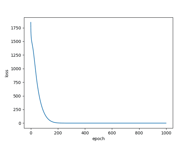
Don’t be shocked by the loss value. If we look at it from a classification perspective, each window has a different label. The loss is bound to be a lot, but thankfully it has dipped to a respectable value.

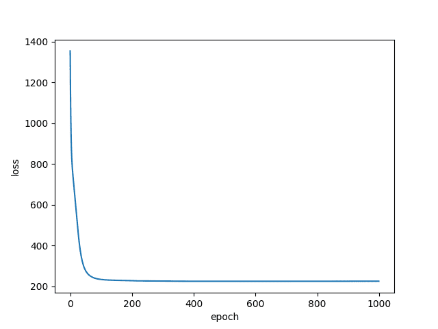
The idea is similar for the Skip-Gram loss, but since we have multiple outputs for a single input, the loss has dipped much faster.

Let’s look at the embedding space itself (Figures 6 and 7).

The CBOW embedding space is fairly scattered, with few visual associations forming. If we look closely, we might find similar contextual words, like years grouped together, etc., but generally, the results aren’t that good.

The Skip-Gram embedding space is much better, as we can see several visual word groupings that have been formed. This shows that in our particular small dataset instance, Skip-Gram has worked much better.

---

---

Summary

Word2Vec is essentially an important milestone in understanding representation learning in NLP. The idea it presents is very intuitive and paves the way for providing a valid solution to the issue of teaching a computer how to understand the meaning of words.

The best part is that the data does most of the work for us. The associations are formed based on how frequently a word appears along with another. Although many better algorithms have popped up in recent years, the impact of embedding spaces can be found in all of them.

---

Citation Information

Chakraborty, D. “Word2Vec: A Study of Embeddings in NLP,” PyImageSearch, P. Chugh, A. R. Gosthipaty, S. Huot, K. Kidriavsteva, R. Raha, and A. Thanki, eds., 2022, https://pyimg.co/2fb0z

@incollection{Chakraborty_2022_Word2Vec,
  author = {Devjyoti Chakraborty},
  title = {{Word2Vec}: A Study of Embeddings in {NLP}},
  booktitle = {PyImageSearch},
  editor = {Puneet Chugh and Aritra Roy Gosthipaty and Susan Huot and Kseniia Kidriavsteva and Ritwik Raha and Abhishek Thanki},
  year = {2022},
  note = {https://pyimg.co/2fb0z},
}

---

To download the source code to this post (and be notified when future tutorials are published here on PyImageSearch), simply enter your email address in the form below!