Training the YOLOv5 Object Detector on a Custom Dataset

---

Table of Contents

---

Training YOLOv5 Object Detector on a Custom Dataset

With the help of Deep Learning, we all know that the field of Computer Vision has proliferated in the last decade. As a result, so many prevalent computer vision problems like image classification, object detection, and segmentation having real industrial use-case started to achieve accuracy like never before. A new benchmark was set every year from 2012. And today, we will look at object detection from a practical perspective.

A custom, annotated image dataset is vital for training the YOLOv5 object detector. It allows us to train the model on specific objects of interest, leading to a detector tailored to our requirements.

Roboflow has free tools for each stage of the computer vision pipeline that will streamline your workflows and supercharge your productivity.

Sign up or Log in to your Roboflow account to access state of the art dataset libaries and revolutionize your computer vision pipeline.

You can start by choosing your own datasets or using our PyimageSearch’s assorted library of useful datasets.

Bring data in any of 40+ formats to Roboflow, train using any state-of-the-art model architectures, deploy across multiple platforms (API, NVIDIA, browser, iOS, etc), and connect to applications or 3rd party tools.

Object detection has various state-of-the-art architectures that can be used off-the-shelf on real-world datasets to detect objects with reasonable accuracy. The only condition is that the test dataset has the same classes as the pre-trained detector.

However, the application you often build might have objects that differ from the pretrained object detector classes. For example, the dataset distribution is very different from where the dataset detector was trained. In such a scenario, we often use the concept of transfer learning, where we use the pre-trained detector and fine-tune it on the newer dataset. In today’s tutorial, you will learn to train the pretrained YOLOv5 object detector on a custom dataset without writing much code.

We will not go into the theoretical details of the YOLOv5 object detector; however, you can check our Introduction to the YOLO Family blog post, where we cover some ground around it.

This lesson is the last in our 7-part series on YOLO:

1. Introduction to the YOLO Family
2. Understanding a Real-Time Object Detection Network: You Only Look Once (YOLOv1)
3. A Better, Faster, and Stronger Object Detector (YOLOv2)
4. Mean Average Precision (mAP) Using the COCO Evaluator
5. An Incremental Improvement with Darknet-53 and Multi-Scale Predictions (YOLOv3)
6. Achieving Optimal Speed and Accuracy in Object Detection (YOLOv4)
7. Training the YOLOv5 Object Detector on a Custom Dataset (today’s tutorial)

To learn how to train a YOLOv5 object detector on a custom dataset, just keep reading.

---

Training YOLOv5 Object Detector on a Custom Dataset

In 2020, Glenn Jocher, the founder and CEO of Ultralytics, released its open-source implementation of YOLOv5 on GitHub. YOLOv5 offers a family of object detection architectures pre-trained on the MS COCO dataset.

Today, YOLOv5 is one of the official state-of-the-art models with tremendous support and is easier to use in production. The best part is that YOLOv5 is natively implemented in PyTorch, eliminating the Darknet framework’s limitations (based on C programming language).

This massive change of YOLO to the PyTorch framework made it easier for the developers to modify the architecture and export to many deployment environments straightforwardly. And not to forget, YOLOv5 is one of the official state-of-the-art models hosted in the Torch Hub showcase.

Table 1 shows the performance (mAP) and speed (FPS) benchmarks of five YOLOv5 variants on the MS COCO validation dataset at 640×640 image resolution on Volta 100 GPU. All five models were trained on the MS COCO training dataset. The model benchmarks are shown in ascending order starting with YOLOv5n (i.e., the nano variant having the smallest model footprint to the largest model, YOLOv5x).

				Speed	Speed	Speed
	size	mAPval	mAPval	CPU b1	V100 b1	V100 b32	params	FLOPs
Model	(pixels)	0.5:0.95	0.5	(ms)	(ms)	(ms)	(M)	@640 (B)
YOLOv5n	640	28.4	46.0	45	6.3	0.6	1.9	4.5
YOLOv5s	640	37.2	56.0	98	6.4	0.9	7.2	16.5
YOLOv5m	640	45.2	63.9	224	8.2	1.7	21.2	49
YOLOv5l	640	48.8	67.2	430	10.1	2.7	46.5	109.1
YOLOv5x	640	50.7	68.9	766	12.1	4.8	86.7	205.7
Table 1: Performance and Speed benchmarks of five YOLOv5 variants on the MS COCO dataset.

Today, we’ll learn how to harness the power of YOLOv5 in the PyTorch framework by transfer learning it on a custom dataset!

---

Configuring Your Development Environment

To follow this guide, you need to clone the Ultralytics YOLOv5 repository and pip install all the necessary packages from requirements.txt.

Luckily, to run the YOLOv5 training, you can just do a pip install on the requirements.txt file, which means that all the libraries are pip-installable!

$ git clone https://github.com/ultralytics/yolov5.git #clone repo
$ cd yolov5/
$ pip install -r requirements.txt #install dependencies

---

Having Problems Configuring Your Development Environment?

All that said, are you:

• Short on time?
• Learning on your employer’s administratively locked system?
• Wanting to skip the hassle of fighting with the command line, package managers, and virtual environments?
• Ready to run the code right now on your Windows, macOS, or Linux system?

Then join PyImageSearch University today!

Gain access to Jupyter Notebooks for this tutorial and other PyImageSearch guides that are pre-configured to run on Google Colab’s ecosystem right in your web browser! No installation required.

And best of all, these Jupyter Notebooks will run on Windows, macOS, and Linux!

---

About the Dataset

For today’s experiment, we will be training the YOLOv5 model on two different datasets, namely the Udacity Self-driving Car dataset and the Vehicles-OpenImages dataset.

These datasets are public, but we download them from Roboflow, which provides a great platform to train your models with various datasets in the Computer Vision domain. Even more interesting is that you can download the datasets in multiple formats like COCO JSON, YOLO Darknet TXT, and YOLOv5 PyTorch. This saves time for writing helper functions for converting the ground-truth annotations to the format required by the model.

---

YOLOv5 Label Format

Since we will train the YOLOv5 PyTorch model, we will download the datasets in YOLOv5 format. The ground-truth annotation format of YOLOv5 is pretty simple (an example is shown in Figure 2), so you could write a script on your own that does that for you. There is one text file with a single line for each bounding box for each image. For example, if there are four objects in one image, the text file would have four rows containing the class label and bounding box coordinates. The format of each row is

class_id center_x center_y width height

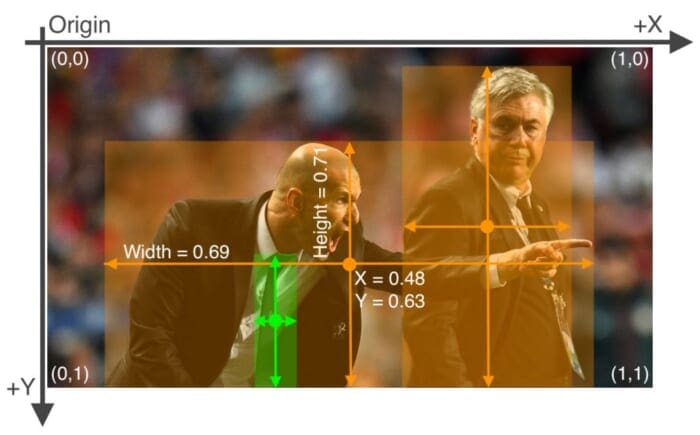
where fields are space-delimited, and the coordinates are normalized from 0 to 1. To convert to normalized xywh from pixel values, divide x & box width by the image’s width and divide y & box height by the image’s height.

---

Vehicles-OpenImages Dataset

This dataset contains only 627 images of various vehicle classes for object detection like Car, Bus, Ambulance, Motorcycle, and Truck. These images are derived from the Open Images open-source computer vision datasets. The dataset falls under the Creative Commons License, which allows you to share and adapt the dataset, and even use it commercially.

Figure 3 shows some sample images from the dataset with ground-truth bounding boxes annotated in green color.

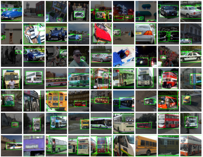
There are 1194 regions of interest (objects) in 627 images, meaning there are at least 1.9 objects per image. Based on the heuristic shown in Figure 4, the car class contributes to more than 50% of the objects. In contrast, the remaining classes: bus, truck, motorcycle, and ambulance, are under-represented relative to the car class.

---

Udacity Self-Driving Car Dataset

Please note that we will not train the YOLOv5 model on this dataset. Instead, we have identified this great dataset for you all as an exercise so that once you are done learning from this tutorial, you can use this dataset for training the object detector.

This dataset is derived from the original Udacity Self-Driving Car Dataset. Unfortunately, the original dataset was missing labels for thousands of pedestrians, bikers, cars, and traffic lights. Hence, Roboflow managed to re-label the dataset to correct errors and omissions.

Figure 5 shows some examples from the dataset and labels missing from the original dataset annotated by Roboflow. If you have worked with autonomous driving urban-scene datasets like Cityscapes, ApolloScape, and Berkeley DeepDrive, you will find this dataset very similar to those.

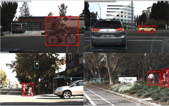
The dataset contains 97,942 labels across 11 classes and 15,000 images. The dataset is available on Roboflow in two different fashions: images with 1920x1200 (download size ~3.1 GB) and a downsampled version with 512x512 (download size ~580 MB) suitable for most. We will use the downsampled version since it is smaller in size and fits our requirements in terms of the network.

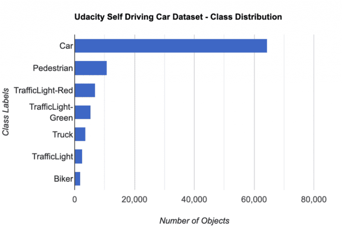
Like the previous Vehicles-OpenImages dataset, this dataset has the most number of objects belonging to the car class (more than 60% of the total objects). Figure 6 shows the distribution of classes in the Udacity Self-Driving Car dataset:

---

Selecting the Model

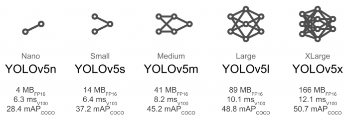
Figure 7 shows five YOLOv5 variants starting with the most miniature YOLOv5 nano model built for running on mobile and embedded devices to YOLOv5 XLarge on the other end of the spectrum. For today’s experiment, we would leverage the base model YOLOv5s, which provides a nice balance between accuracy and speed.

---

YOLOv5 Training

This section is the heart of today’s tutorial, where we will cover most of the things, starting with

• Downloading the dataset
• Creating the data configuration
• Training the YOLOv5 model
• Visualizing the YOLOv5 model artifacts
• Quantitative results
• Freeze initial layers and fine-tune the remaining layers
• Results

---

Downloading the Vehicles-OpenImages Dataset

# Download the vehicles-open image dataset
!mkdir vehicles_open_image
%cd vehicles_open_image
!curl -L "https://public.roboflow.com/ds/2Tb6yXY8l8?key=Eg82WpxUEr" > vehicles.zip 
!unzip vehicles.zip
!rm vehicles.zip

On Lines 2 and 3, we create the vehicles_open_image directory and cd into the directory where we download the dataset. Then, on Line 4, we use the curl command and pass the dataset URL we got from here. Finally, we unzip the dataset and remove the zip file on Lines 5 and 6.

Let’s look at the contents of the vehicles_open_image folder:

$tree /content/vehicles_open_image -L 2
/content/vehicles_open_image
├── data.yaml
├── README.dataset.txt
├── README.roboflow.txt
├── test
│   ├── images
│   └── labels
├── train
│   ├── images
│   └── labels
└── valid
    ├── images
    └── labels

9 directories, 3 files

The parent directory has three files, out of which only data.yaml is essential, and three sub-directories:

• data.yaml: It has the data-related configurations like the train and valid data directory path, the total number of classes in the dataset, and the name of each class
• train: Training images along with training labels
• valid: Validation images with annotations
• test: Test images and labels. Assessing your model’s performance becomes easy if test data with labels are available.

---

Configuration Setup

Next, we will edit the data.yaml file to have the path and absolute path for train and valid images.

# Create configuration
import yaml
config = {'path': '/content/vehicles_open_image',
         'train': '/content/vehicles_open_image/train',
         'val': '/content/vehicles_open_image/valid',
         'nc': 5,
         'names': ['Ambulance', 'Bus', 'Car', 'Motorcycle', 'Truck']}
 
with open("data.yaml", "w") as file:
   yaml.dump(config, file, default_flow_style=False)

On Line 2, we import the yaml module, which would allow us to save the data.yaml configuration file in .yaml format. Then from Lines 3-7, we define the data path, train, validation, number of classes, and class names in a config variable. So config is a dictionary.

Finally, on Lines 9 and 10, we open the existing data.yaml file that was downloaded along with the dataset, overwrite it with the contents in config, and store it on the disk.

---

YOLOv5 Training Hyperparameters and Model Configuration

YOLOv5 has about 30 hyperparameters used for various training settings. These are defined in hyp.scratch-low.yaml for low-augmentation COCO training from scratch, placed in the /data directory. The training data hyperparameters are shown below, which are very important for producing good results, so make sure to initialize these values properly before starting the training. For this tutorial, we would simply use the default values, which are optimized for YOLOv5 COCO training from scratch.

As you can see, it has learning rate, weight_decay, and iou_t (IoU training threshold), to name a few, and some data augmentation hyperparameters like translate, scale, mosaic, mixup, and copy_paste. A mixup:0.0 means the mixup data augmentation should not be applied.

lr0: 0.01  # initial learning rate (SGD=1E-2, Adam=1E-3)
lrf: 0.01  # final OneCycleLR learning rate (lr0 * lrf)
momentum: 0.937  # SGD momentum/Adam beta1
weight_decay: 0.0005  # optimizer weight decay 5e-4
warmup_epochs: 3.0  # warmup epochs (fractions ok)
warmup_momentum: 0.8  # warmup initial momentum
warmup_bias_lr: 0.1  # warmup initial bias lr
box: 0.05  # box loss gain
cls: 0.5  # cls loss gain
cls_pw: 1.0  # cls BCELoss positive_weight
obj: 1.0  # obj loss gain (scale with pixels)
obj_pw: 1.0  # obj BCELoss positive_weight
iou_t: 0.20  # IoU training threshold
anchor_t: 4.0  # anchor-multiple threshold
# anchors: 3  # anchors per output layer (0 to ignore)
fl_gamma: 0.0  # focal loss gamma (efficientDet default gamma=1.5)
hsv_h: 0.015  # image HSV-Hue augmentation (fraction)
hsv_s: 0.7  # image HSV-Saturation augmentation (fraction)
hsv_v: 0.4  # image HSV-Value augmentation (fraction)
degrees: 0.0  # image rotation (+/- deg)
translate: 0.1  # image translation (+/- fraction)
scale: 0.5  # image scale (+/- gain)
shear: 0.0  # image shear (+/- deg)
perspective: 0.0  # image perspective (+/- fraction), range 0-0.001
flipud: 0.0  # image flip up-down (probability)
fliplr: 0.5  # image flip left-right (probability)
mosaic: 1.0  # image mosaic (probability)
mixup: 0.0  # image mixup (probability)
copy_paste: 0.0  # segment copy-paste (probability)

Next, you can briefly look at the structure of the YOLOv5s network architecture, though you would hardly modify the model configuration file, unlike the training data hyperparameters. It has nc set to 80 for MS COCO dataset, backbone for feature extraction, followed by head for detection.

# Parameters
nc: 80  # number of classes
depth_multiple: 0.33  # model depth multiple
width_multiple: 0.50  # layer channel multiple
anchors:
  - [10,13, 16,30, 33,23]  # P3/8
  - [30,61, 62,45, 59,119]  # P4/16
  - [116,90, 156,198, 373,326]  # P5/32

# YOLOv5 v6.0 backbone
backbone:
  # [from, number, module, args]
  [[-1, 1, Conv, [64, 6, 2, 2]],  # 0-P1/2
   [-1, 1, Conv, [128, 3, 2]],  # 1-P2/4
   [-1, 3, C3, [128]],
   [-1, 1, Conv, [256, 3, 2]],  # 3-P3/8
   [-1, 6, C3, [256]],
   [-1, 1, Conv, [512, 3, 2]],  # 5-P4/16
   [-1, 9, C3, [512]],
   [-1, 1, Conv, [1024, 3, 2]],  # 7-P5/32
   [-1, 3, C3, [1024]],
   [-1, 1, SPPF, [1024, 5]],  # 9
  ]

# YOLOv5 v6.0 head
head:
  [[-1, 1, Conv, [512, 1, 1]],
   [-1, 1, nn.Upsample, [None, 2, 'nearest']],
   [[-1, 6], 1, Concat, [1]],  # cat backbone P4
   [-1, 3, C3, [512, False]],  # 13

   [-1, 1, Conv, [256, 1, 1]],
   [-1, 1, nn.Upsample, [None, 2, 'nearest']],
   [[-1, 4], 1, Concat, [1]],  # cat backbone P3
   [-1, 3, C3, [256, False]],  # 17 (P3/8-small)

   [-1, 1, Conv, [256, 3, 2]],
   [[-1, 14], 1, Concat, [1]],  # cat head P4
   [-1, 3, C3, [512, False]],  # 20 (P4/16-medium)

   [-1, 1, Conv, [512, 3, 2]],
   [[-1, 10], 1, Concat, [1]],  # cat head P5
   [-1, 3, C3, [1024, False]],  # 23 (P5/32-large)

   [[17, 20, 23], 1, Detect, [nc, anchors]],  # Detect(P3, P4, P5)
  ]

---

Training the YOLOv5s Model

We are almost ready to train the YOLOv5 model, and as discussed above, we will be training the YOLOv5s model. However, before we run the training, let’s define a few parameters:

SIZE = 640
BATCH_SIZE = 32
EPOCHS = 20
MODEL = "yolov5s"
WORKERS = 1
PROJECT = "vehicles_open_image_pyimagesearch"
RUN_NAME = f"{MODEL}_size{SIZE}_epochs{EPOCHS}_batch{BATCH_SIZE}_small"

We define a few standard model parameters:

• SIZE: Image size or network input while training. The images will be resized to this value before being fed to the network. The preprocessing pipeline would resize them to 640 pixels.
• BATCH_SIZE: Number of images fed as a single batch into the network for a forward pass. You can modify it according to the GPU memory available. We have set it to 32.
• EPOCHS: Number of times we want to train the model on the full dataset.
• MODEL: The base model we want to use for training. We use the small model yolov5s from the YOLOv5 family.
• WORKERS: Maximum Dataloader workers to be used.
• PROJECT: This will create a project directory inside the current directory (yolov5).
• RUN_NAME: Each time you run this model, it will create a sub-directory under the project directory, which would have a lot of information on the model like weights, sample input images, a few validation predictions outputs, metrics plot, etc.

!python train.py --img {SIZE}\
               --batch {BATCH_SIZE}\
               --epochs {EPOCHS}\
               --data ../vehicles_open_image/data.yaml\
               --weights {MODEL}.pt\
               --workers {WORKERS}\
               --project {PROJECT}\
               --name {RUN_NAME}\
               --exist-ok

If there are no errors, the training will start as shown below. The logs indicate that the YOLOv5 model would train with Torch version 1.11 on a Tesla T4 GPU; along with that, it also shows the hyperparameters initialized.

The yolov5s.pt weights are downloaded, which means that the YOLOv5s model is initialized with the parameters trained with the MS COCO dataset. Finally, we can see that two epochs have been completed with a mAP@0.5=0.237.

github: up to date with https://github.com/ultralytics/yolov5 ✅
YOLOv5 ? v6.1-236-gdcf8073 Python-3.7.13 torch-1.11.0+cu113 CUDA:0 (Tesla T4, 15110MiB)
hyperparameters: lr0=0.01, lrf=0.01, momentum=0.937, weight_decay=0.0005, warmup_epochs=3.0, warmup_momentum=0.8, warmup_bias_lr=0.1, box=0.05, cls=0.5, cls_pw=1.0, obj=1.0, obj_pw=1.0, iou_t=0.2, anchor_t=4.0, fl_gamma=0.0, hsv_h=0.015, hsv_s=0.7, hsv_v=0.4, degrees=0.0, translate=0.1, scale=0.5, shear=0.0, perspective=0.0, flipud=0.0, fliplr=0.5, mosaic=1.0, mixup=0.0, copy_paste=0.0
Weights & Biases: run 'pip install wandb' to automatically track and visualize YOLOv5 ? runs (RECOMMENDED)
TensorBoard: Start with 'tensorboard --logdir parking_lot_pyimagesearch', view at http://localhost:6006/
Downloading https://ultralytics.com/assets/Arial.ttf to /root/.config/Ultralytics/Arial.ttf...
100% 755k/755k [00:00<00:00, 18.0MB/s]
YOLOv5 temporarily requires wandb version 0.12.10 or below. Some features may not work as expected.
Downloading https://github.com/ultralytics/yolov5/releases/download/v6.1/yolov5s.pt to yolov5s.pt...
100% 14.1M/14.1M [00:00<00:00, 125MB/s]

Overriding model.yaml nc=80 with nc=5
Logging results to parking_lot_pyimagesearch/yolov5s_size640_epochs20_batch32_simple
Starting training for 20 epochs...

     Epoch   gpu_mem       box       obj       cls    labels  img_size
      0/19     7.36G   0.09176   0.03736   0.04355        31       640: 100% 28/28 [00:28<00:00,  1.03s/it]
               Class     Images     Labels          P          R     mAP@.5 mAP@.5:.95: 100% 4/4 [00:03<00:00,  1.04it/s]
                 all        250        454      0.352      0.293      0.185      0.089

     Epoch   gpu_mem       box       obj       cls    labels  img_size
      1/19     8.98G   0.06672   0.02769   0.03154        45       640: 100% 28/28 [00:25<00:00,  1.09it/s]
               Class     Images     Labels          P          R     mAP@.5 mAP@.5:.95: 100% 4/4 [00:05<00:00,  1.45s/it]
                 all        250        454      0.271      0.347      0.237     0.0735

Voila! With this, you have learned to train an object detector on a custom dataset you downloaded from Roboflow. Isn’t that amazing?

Even more exciting is that YOLOv5 logs the model artifacts inside the runs directory, which we will look at in the next section.

Once the training is complete, you will see the output similar to the one shown below:

​​    Epoch   gpu_mem       box       obj       cls    labels  img_size
     19/19     7.16G   0.02747   0.01736  0.004772        46       640: 100% 28/28 [01:03<00:00,  2.27s/it]
               Class     Images     Labels          P          R     mAP@.5 mAP@.5:.95: 100% 4/4 [00:05<00:00,  1.42s/it]
                 all        250        454      0.713      0.574      0.606      0.416

20 epochs completed in 0.386 hours.
Optimizer stripped from runs/train/exp/weights/last.pt, 14.5MB
Optimizer stripped from runs/train/exp/weights/best.pt, 14.5MB

Validating runs/train/exp/weights/best.pt...
Fusing layers... 
Model summary: 213 layers, 7023610 parameters, 0 gradients, 15.8 GFLOPs
               Class     Images     Labels          P          R     mAP@.5 mAP@.5:.95: 100% 4/4 [00:08<00:00,  2.23s/it]
                 all        250        454      0.715      0.575      0.606      0.416
           Ambulance        250         64      0.813      0.814      0.853      0.679
                 Bus        250         46      0.771      0.652      0.664       0.44
                 Car        250        238      0.653      0.496      0.518      0.354
          Motorcycle        250         46      0.731      0.478      0.573      0.352
               Truck        250         60      0.608      0.433      0.425      0.256

The above results show that the YOLOv5s model achieved an mAP of 0.606@0.5 IoU and 0.416@0.5:0.95 IoU in all classes. It also indicates class-wise mAP, and the model achieved the best score for the Ambulance class (i.e., 0.853 mAP@0.5 IoU). The model took 23.16 minutes to complete the training for 20 epochs on a Tesla T4 or Tesla K80.

---

Visualizing Model Artifacts

Now that we are done training our model, let’s look at the results generated inside the yolov5/vehicles_open_pyimagesearch_model directory.

All training results are logged by default to yolov5/runs/train with a new incrementing directory created for each run as runs/train/exp, runs/train/exp1, etc. However, while training the model, we passed the PROJECT and the RUN_NAME, so in this case, it does not create the default directory to log the training results. Hence, in this experiment runs is parking_lot_pyimagesearch.

Next, let’s look at the files created in the experiment.

$tree parking_lot_pyimagesearch/yolov5s_size640_epochs20_batch32_small/
parking_lot_pyimagesearch/yolov5s_size640_epochs20_batch32_small/
├── confusion_matrix.png
├── events.out.tfevents.1652810418.f70b01be1223.864.0
├── F1_curve.png
├── hyp.yaml
├── labels_correlogram.jpg
├── labels.jpg
├── opt.yaml
├── P_curve.png
├── PR_curve.png
├── R_curve.png
├── results.csv
├── results.png
├── train_batch0.jpg
├── train_batch1.jpg
├── train_batch2.jpg
├── val_batch0_labels.jpg
├── val_batch0_pred.jpg
├── val_batch1_labels.jpg
├── val_batch1_pred.jpg
├── val_batch2_labels.jpg
├── val_batch2_pred.jpg
└── weights
    ├── best.pt
    └── last.pt

1 directory, 23 files

On Line 1, we use the tree command followed by the PROJECT and RUN_NAME, displaying various evaluation metrics and weights files for the trained object detector. As we can observe, it has a precision curve, recall curve, precision-recall curve, confusion matrix, prediction on validation images, and finally, the weights file in PyTorch format.

Let’s now look at a few images from the runs directory.

Figure 8 shows the training images batch with Mosaic data augmentation. There are 16 images clubbed together; if we pick one image from the 3rd row 1st column, then we can see that the image is a combination of four different images. We explain the concept of Mosaic data augmentation in the YOLOv4 post, so do check that out if you haven’t already.

Next, we look at the results.png, which comprises training and validation loss for bounding box, objectness, and classification. It also has the metrics: precision, recall, mAP@0.5, and mAP@0.5:0.95 for training (Figure 9).

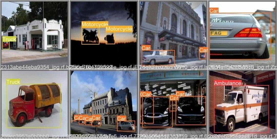
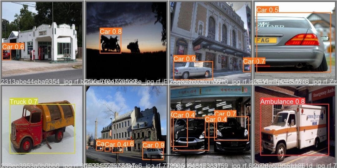
Figure 10 shows the ground-truth images and the YOLOv5s model prediction on the Vehicles-OpenImages dataset. From the two images below, it is clear that the model did a great job detecting the objects. Unfortunately, the model failed to detect a bike in the second image and a car in the sixth image. And misclassified a truck as a car in the first image, but this was a tough one to crack as it’s even difficult for the human to predict it correctly. But overall, it did great on these images.

---

Freeze Initial Layers and Fine-Tune Remaining Layers

We learned how to train an object detector that was pretrained on the MS COCO dataset, which means we fine-tuned the model parameters (all layers) on the Vehicles-OpenImages dataset. But the question is, do we need to train all the model layers on the new dataset? Maybe not, since the pretrained model has been trained on a large, well-curated MS COCO dataset.

The benefit of freezing layers when often fine-tuning a model on a custom dataset reduces the training time. If the custom dataset is not too complex, then you can expect, if not the same, but comparable accuracies. When we compare the two models’ training times, you will see for yourself.

In this section, we will again train or fine-tune the YOLOv5s model on the Vehicles-OpenImages dataset but freeze the initial 11 layers of the network, unlike before, where we fine-tune all the detector layers. Thanks to the creators of YOLOv5, freezing the model layers is very easy. But, first, we must pass the --freeze argument with the layer numbers we would like to freeze in the model.

Let’s now train the model by executing the train.py script. First, we change the --name, that is, the run name to freeze_layers, pass the --freeze parameter, and all other parameters are the same.

!python train.py --img {SIZE}\
               --batch {BATCH_SIZE}\
               --epochs {EPOCHS}\
               --data ../vehicles_open_image/data.yaml\
               --weights {MODEL}.pt\
               --workers {WORKERS}\
               --project {PROJECT}\
               --name freeze_layers\
               --exist-ok\
               --freeze 0 1 2 3 4 5 6 7 8 9 10

The output below is produced when you run the training script; as you can see, the first 11 layers of the network are shown with a freezing prefix which means that the parameters (weights and biases) for these layers would remain constant. At the same time, the remaining 15 layers would be fine-tuned on the custom dataset.

That being said, let us look at the results now!

freezing model.0.conv.weight
freezing model.0.bn.weight
freezing model.0.bn.bias
freezing model.1.conv.weight
freezing model.1.bn.weight
freezing model.1.bn.bias
.
.
.
.
freezing model.10.conv.weight
freezing model.10.bn.weight
freezing model.10.bn.bias

We can observe from the below output that 20 epochs were completed in only 0.158 hours (i.e., 9.48 mins), and the model we fine-tuned with none of the layers frozen took 23.16 minutes. Wow! That’s close to a 2.5X reduction in time.

But hold on, let’s look at the mAP of this model shown for all classes and class-wise.

With 11 layers frozen, the model achieved 0.551 mAP@0.5 IoU and 0.336 mAP@0.5:0.95 IoU. There is definitely a difference between the accuracies of the two models but not too significant.

20 epochs completed in 0.158 hours.
Optimizer stripped from parking_lot_pyimagesearch/freeze_layers/weights/last.pt, 14.5MB
Optimizer stripped from parking_lot_pyimagesearch/freeze_layers/weights/best.pt, 14.5MB

Validating parking_lot_pyimagesearch/freeze_layers/weights/best.pt...
Fusing layers... 
Model summary: 213 layers, 7023610 parameters, 0 gradients, 15.8 GFLOPs
               Class     Images     Labels          P          R     mAP@.5 mAP@.5:.95: 100% 4/4 [00:04<00:00,  1.25s/it]
                 all        250        454      0.579      0.585      0.551      0.336
           Ambulance        250         64      0.587      0.688      0.629      0.476
                 Bus        250         46      0.527      0.696      0.553      0.304
                 Car        250        238      0.522      0.462      0.452      0.275
          Motorcycle        250         46      0.733      0.478      0.587      0.311
               Truck        250         60      0.527        0.6      0.533      0.313

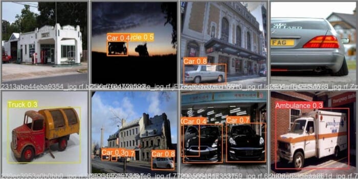
Finally, in Figure 11, we can see the detector prediction on the validation images. The results clearly show that they are not as good as the detector trained with all layers. For example, it misses the object in the first image, in the second image, it misclassifies a motorcycle with a car, in the fourth image fails to detect the car, and even in the sixth image, it sees only three cars. Maybe training for a bit more epochs or freezing fewer layers could improve the detector’s performance.

---

---

Summary

Congratulations on making it this far! Let’s quickly summarize what we learned in this tutorial.

1. We started by giving a brief overview of YOLOv5 and discussed the performance and speed benchmarks of YOLOv5 variants.
2. Then we discussed the two datasets: Vehicles-OpenImages dataset and Udacity Self-Driving Car dataset. Along with that we also covered the YOLOv5 ground-truth annotation format.
3. After finalizing the YOLOv5 model variant for training we dived into the hands-on part of the tutorial where we covered aspects like downloading the dataset, creating configuration.yaml for the given data, and training and visualizing the YOLOv5 model artifacts.
4. Finally, we trained the YOLOv5 model for the second time but with the initial 11 layers of the model frozen and compared the results with the YOLOv5 model trained fully.

---

Citation Information

Sharma, A. “Training the YOLOv5 Object Detector on a Custom Dataset,” PyImageSearch, D. Chakraborty, P. Chugh, A. R. Gosthipaty, S. Huot, K. Kidriavsteva, R. Raha, and A. Thanki, eds., 2022, https://pyimg.co/fq0a3

@incollection{Sharma_2022_Custom_Dataset,
  author = {Aditya Sharma},
  title = {Training the {YOLOv5} Object Detector on a Custom Dataset},
  booktitle = {PyImageSearch},
  editor = {Devjyoti Chakraborty and Puneet Chugh and Aritra Roy Gosthipaty and Susan Huot and Kseniia Kidriavsteva and Ritwik Raha and Abhishek Thanki},
  year = {2022},
  note = {https://pyimg.co/fq0a3},
}

---

To download the source code to this post (and be notified when future tutorials are published here on PyImageSearch), simply enter your email address in the form below!