Introduction to Neural Networks

We’ll study the fundamentals of neural networks in depth. We’ll start with a discussion of artificial neural networks and how they are inspired by the real-life biological neural networks in our own bodies. From there, we’ll review the classic Perceptron algorithm and the role it has played in neural network history.

Building on the Perceptron, we’ll also study the backpropagation algorithm, the cornerstone of modern neural learning — without backpropagation, we would be unable to efficiently train our networks. We’ll also implement backpropagation with Python from scratch, ensuring we understand this important algorithm.

Of course, modern neural network libraries such as Keras already have (highly optimized) backpropagation algorithms built-in. Implementing backpropagation by hand each time we wished to train a neural network would be like coding a linked list or hash table data structure from scratch each time we worked on a general purpose programming problem — not only is it unrealistic, but it’s also a waste of our time and resources. In order to streamline the process, I’ll demonstrate how to create standard feedforward neural networks using the Keras library.

Finally, we’ll discuss the four ingredients you’ll need when building any neural network.

Neural Network Basics

Before we can work with Convolutional Neural Networks, we first need to understand the basics of neural networks. We’ll review:

• Artificial Neural Networks and their relation to biology.
• The seminal Perceptron algorithm.
• The backpropagation algorithm and how it can be used to train multi-layer neural networks efficiently.
• How to train neural networks using the Keras library.

By the time you finish, you’ll have a strong understanding of neural networks and be able to move on to the more advanced Convolutional Neural Networks.

Introduction to Neural Networks

Neural networks are the building blocks of deep learning systems. In order to be successful at deep learning, we need to start by reviewing the basics of neural networks, including architecture, node types, and algorithms for “teaching” our networks.

We’ll start with a high-level overview of neural networks and the motivation behind them, including their relation to biology in the human mind. From there we’ll discuss the most common type of architecture, feedforward neural networks. We’ll also briefly discuss the concept of neural learning and how it will later relate to the algorithms we use to train neural networks.

What are Neural Networks?

Many tasks that involve intelligence, pattern recognition, and object detection are extremely difficult to automate, yet seem to be performed easily and naturally by animals and young children. For example, how does your family dog recognize you, the owner, versus a complete and total stranger? How does a small child learn to recognize the difference between a school bus and a transit bus? And how do our own brains subconsciously perform complex pattern recognition tasks each and every day without us even noticing?

The answer lies within our own bodies. Each of us contains a real-life biological neural network that is connected to our nervous systems — this network is made up of a large number of interconnected neurons (nerve cells).

The word “neural” is the adjective form of “neuron,” and “network” denotes a graph-like structure; therefore, an “Artificial Neural Network” is a computation system that attempts to mimic (or at least, is inspired by) the neural connections in our nervous system. Artificial neural networks are also referred to as “neural networks” or “artificial neural systems.” It is common to abbreviate Artificial Neural Network and refer to them as “ANN” or simply “NN” — I will be using both of the abbreviations.

For a system to be considered an NN, it must contain a labeled, directed graph structure where each node in the graph performs some simple computation. From graph theory, we know that a directed graph consists of a set of nodes (i.e., vertices) and a set of connections (i.e., edges) that link together pairs of nodes. In Figure 1, we can see an example of such an NN graph.

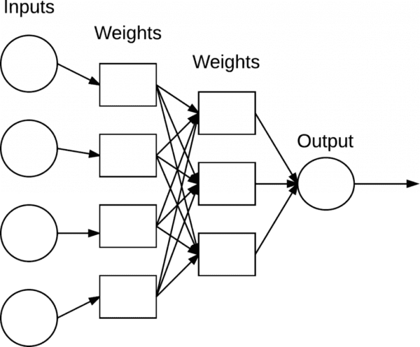
Each node performs a simple computation. Each connection then carries a signal (i.e., the output of the computation) from one node to another, labeled by a weight indicating the extent to which the signal is amplified or diminished. Some connections have large, positive weights that amplify the signal, indicating that the signal is very important when making a classification. Others have negative weights, diminishing the strength of the signal, thus specifying that the output of the node is less important in the final classification. We call such a system an Artificial Neural Network if it consists of a graph structure (like in Figure 1) with connection weights that are modifiable using a learning algorithm.

Relation to Biology

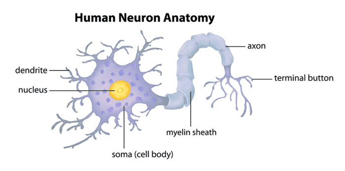
Our brains are composed of approximately 10 billion neurons, each connected to about 10,000 other neurons. The cell body of the neuron is called the soma, where the inputs (dendrites) and outputs (axons) connect soma to other soma (Figure 2).

Each neuron receives electrochemical inputs from other neurons at their dendrites. If these electrical inputs are sufficiently powerful to activate the neuron, then the activated neuron transmits the signal along its axon, passing it along to the dendrites of other neurons. These attached neurons may also fire, thus continuing the process of passing the message along.

The key takeaway here is that a neuron firing is a binary operation — the neuron either fires or it doesn’t fire. There are no different “grades” of firing. Simply put, a neuron will only fire if the total signal received at the soma exceeds a given threshold.

However, keep in mind that ANNs are simply inspired by what we know about the brain and how it works. The goal of deep learning is not to mimic how our brains function, but rather take the pieces that we understand and allow us to draw similar parallels in our own work. At the end of the day, we do not know enough about neuroscience and the deeper functions of the brain to be able to correctly model how the brain works — instead, we take our inspirations and move on from there.

Artificial Models

Let’s start by taking a look at a basic NN that performs a simple weighted summation of the inputs in Figure 3. The values x₁, x₂, and, x₃ are the inputs to our NN and typically correspond to a single row (i.e., data point) from our design matrix. The constant value 1 is our bias that is assumed to be embedded into the design matrix. We can think of these inputs as the input feature vectors to the NN.

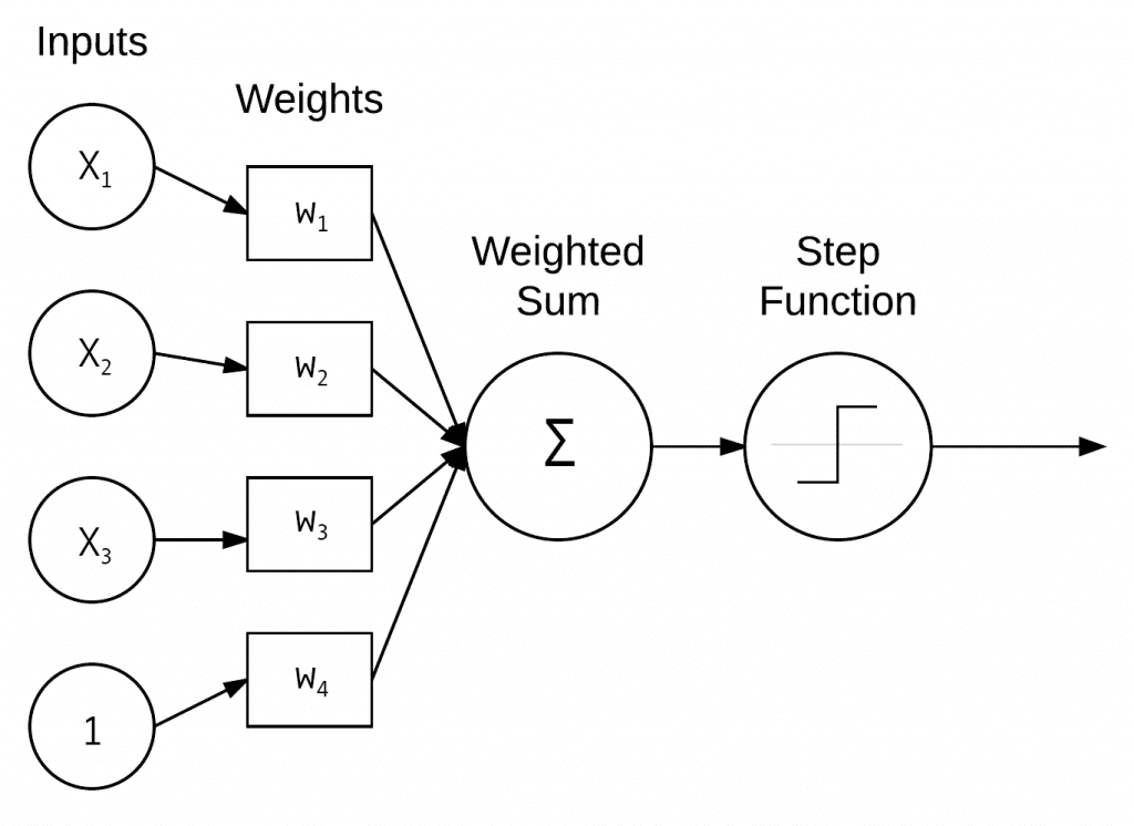
In practice, these inputs could be vectors used to quantify the contents of an image in a systematic, predefined way (e.g., color histograms, Histogram of Oriented Gradients, Local Binary Patterns, etc.). In the context of deep learning, these inputs are the raw pixel intensities of the images themselves.

Each x is connected to a neuron via a weight vector W consists of w₁, w₂, …, w_n, meaning that for each input x we also have an associated weight w.

Finally, the output node on the right of Figure 3 takes the weighted sum, applies an activation function f (used to determine if the neuron “fires” or not), and outputs a value. Expressing the output mathematically, you’ll typically encounter the following three forms:

• f(w₁x₁ +w₂x₂ + ··· +w_nx_n)
• f(∑ⁿ_i=1w_ix_i)
• Or simply, f(net), where net = ∑ⁿ_i=1w_ix_i

Regardless of how the output value is expressed, understand that we are simply taking the weighted sum of inputs, followed by applying an activation function f.

Activation Functions

The most simple activation function is the “step function,” used by the Perceptron algorithm.

As we can see from the equation above, this is a very simple threshold function. If the weighted sum ∑ⁿ_i=1w_ix_i > 0, we output 1, otherwise, we output 0.

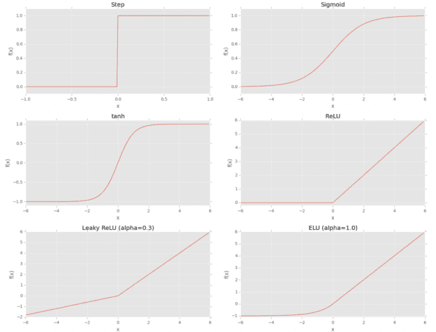
Plotting input values along the x-axis and the output of f(net) along the y-axis, we can see why this activation function received its name (Figure 4, top-left). The output of f is always zero when net is less than or equal zero. If net is greater than zero, then f will return one. Thus, this function looks like a stair step, not dissimilar to the stairs you walk up and down every day.

However, while being intuitive and easy to use, the step function is not differentiable, which can lead to problems when applying gradient descent and training our network.

Instead, a more common activation function used in the history of NN literature is the sigmoid function (Figure 4, top-right), which follows the equation:

(1)

The sigmoid function is a better choice for learning than the simple step function since it:

1. Is continuous and differentiable everywhere.
2. Is symmetric around the y-axis.
3. Asymptotically approaches its saturation values.

The primary advantage here is that the smoothness of the sigmoid function makes it easier to devise learning algorithms. However, there are two big problems with the sigmoid function:

1. The outputs of the sigmoid are not zero centered.
2. Saturated neurons essentially kill the gradient, since the delta of the gradient will be extremely small.

The hyperbolic tangent, or tanh (with a similar shape of the sigmoid) was also heavily used as an activation function up until the late 1990s (Figure 4, mid-left): The equation for tanh follows:

(2) f(z) = tanh(z) = (e^z −e^−z) / (e^z +e^−z)

The tanh function is zero centered, but the gradients are still killed when neurons become saturated.

We now know there are better choices for activation functions than the sigmoid and tanh functions. Specifically, the work of Hahnloser et al. in their 2000 paper, Digital selection and analogue amplification coexist in a cortex-inspired silicon circuit, introduced the Rectified Linear Unit (ReLU), defined as:

(3) f(x) = max(0, x)

ReLUs are also called “ramp functions” due to how they look when plotted (Figure 4, mid-right). Notice how the function is zero for negative inputs but then linearly increases for positive values. The ReLU function is not saturable and is also extremely computationally efficient.

Empirically, the ReLU activation function tends to outperform both the sigmoid and tanh functions in nearly all applications. Combined with the work of Hahnloser and Seung in their follow-up 2003 paper Permitted and Forbidden Sets in Symmetric Threshold-Linear Networks, it was found that the ReLU activation function has stronger biological motivations than the previous families of activation functions, including more complete mathematical justifications.

As of 2015, ReLU is the most popular activation function used in deep learning (LeCun, Bengio, and Hinton, 2015). However, a problem arises when we have a value of zero — the gradient cannot be taken.

A variant of ReLUs, called Leaky ReLUs (Maas, Hannun, and Ng, 2013) allow for a small, non-zero gradient when the unit is not active:

Plotting this function in Figure 4 (bottom-left), we can see that the function is indeed allowed to take on a negative value, unlike traditional ReLUs which “clamp” the function output at zero.

Parametric ReLUs, or PReLUs for short (He, Zhang, Ren, and Sun, 2015), build on Leaky ReLUs and allow the parameter α to be learned on an activation-by-activation basis, implying that each node in the network can learn a different “coefficient of leakage” separate from the other nodes.

Finally, we also have Exponential Linear Units (ELUs) introduced by Clevert et al. in their 2015 paper, Fast and Accurate Deep Learning by Exponential Linear Units (ELUs):

The value of α is constant and set when the network architecture is instantiated — this is unlike PReLUs where α is learned. A typical value for α is α = 1.0. Figure 4 (bottom-right) visualizes the ELU activation function.

Through the work of Clevert et al. (and my own anecdotal experiments), ELUs often obtain higher classification accuracy than ReLUs. ELUs rarely, if ever perform worse than your standard ReLU function.

Which Activation Function Do I Use?

Given the popularity of the most recent incarnation of deep learning, there has been an associated explosion in activation functions. Due to the number of choices of activation functions, both modern (ReLU, Leaky ReLU, ELU, etc.) and “classical” ones (step, sigmoid, tanh, etc.), it may appear to be a daunting, perhaps even overwhelming task to select an appropriate activation function.

However, in nearly all situations, I recommend starting with a ReLU to obtain a baseline accuracy (as do most papers published in the deep learning literature). From there you can try swapping out your standard ReLU for a Leaky ReLU variant.

My personal preference is to start with a ReLU, tune my network and optimizer parameters (architecture, learning rate, regularization strength, etc.), and note the accuracy. Once I am reasonably satisfied with the accuracy, I swap in an ELU and often notice a 1−5% improvement in classification accuracy depending on the dataset. Again, this is only my anecdotal advice. You should run your own experiments and note your findings, but as a general rule of thumb, start with a normal ReLU and tune the other parameters in your network — then swap in some of the more “exotic” ReLU variants.

Feedforward Network Architectures

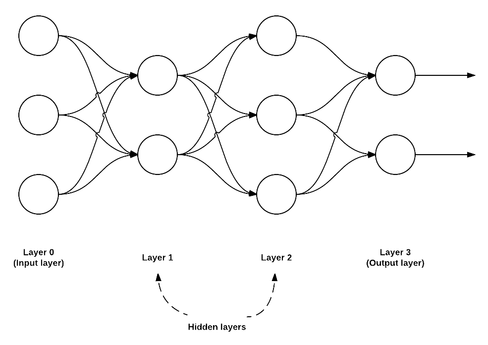
While there are many, many different NN architectures, the most common architecture is the feedforward network, as presented in Figure 5.

In this type of architecture, a connection between nodes is only allowed from nodes in layer i to nodes in layer i+1 (hence the term, feedforward). There are no backward or inter-layer connections allowed. When feedforward networks include feedback connections (output connections that feed back into the inputs) they are called recurrent neural networks.

We focus on feedforward neural networks as they are the cornerstone of modern deep learning applied to computer vision. Convolutional Neural Networks are simply a special case of feedforward neural networks.

To describe a feedforward network, we normally use a sequence of integers to quickly and concisely denote the number of nodes in each layer. For example, the network in Figure 5 is a 3-2-3-2 feedforward network:

Layer 0 contains 3 inputs, our x_i values. These could be raw pixel intensities of an image or a feature vector extracted from the image.

Layers 1 and 2 are hidden layers containing 2 and 3 nodes, respectively.

Layer 3 is the output layer or the visible layer — there is where we obtain the overall output classification from our network. The output layer typically has as many nodes as class labels; one node for each potential output. For example, if we were to build an NN to classify handwritten digits, our output layer would consist of 10 nodes, one for each digit 0-9.

Neural Learning

Neural learning refers to the method of modifying the weights and connections between nodes in a network. Biologically, we define learning in terms of Hebb’s principle:

When an axon of cell A is near enough to excite cell B, and repeatedly or persistently takes place in firing it, some growth process or metabolic change takes place in one or both cells such that A’s efficiency, as one of the cells firing B, is increased.

— Donald Hebb (1949)

In terms of ANNs, this principle implies that there should be an increase in the strength of connections between nodes that have similar outputs when presented with the same input. We call this correlation learning because the strength of the connections between neurons eventually represents the correlation between outputs.

What are Neural Networks Used For?

Neural Networks can be used in both supervised, unsupervised, and semi-supervised learning tasks, provided the appropriate architecture is utilized, of course. Common applications of NN include classification, regression, clustering, vector quantization, pattern association, and function approximation, just to name a few.

In fact, for nearly every facet of machine learning, NNs have been applied in some form or another. We’ll be using NNs for computer vision and image classification.

A Summary of Neural Network Basics

Today, we reviewed the basics of Artificial Neural Networks (ANNs, or simply NNs). We started by examining the biological motivation behind ANNs and then learned how we can mathematically define a function to mimic the activation of a neuron (i.e., the activation function).

Based on this model of a neuron, we are able to define the architecture of a network consisting of (at a bare minimum), an input layer and an output layer. Some network architectures may include multiple hidden layers between the input and output layers. Finally, each layer can have one or more nodes. Nodes in the input layer do not contain an activation function (they are “where” the individual pixel intensities of our image are inputted); however, nodes in both the hidden and output layers do contain an activation function.

We also reviewed three popular activation functions: sigmoid, tanh, and ReLU (and its variants).

Traditionally the sigmoid and tanh functions have been used to train networks; however, since Hahnloser et al.’s 2000 paper, the ReLU function has been used more often.

In 2015, ReLU is by far the most popular activation function used in deep learning architectures (LeCun, Bengio, and Hinton, 2015). Based on the success of ReLU, we also have Leaky ReLUs, a variant of ReLUs that seek to improve network performance by allowing the function to take on a negative value. The Leaky ReLU family of functions consists of your standard leaky ReLU variant, PReLUs, and ELUs.

Finally, it’s important to note that even though we are focusing on deep learning strictly in the context of image classification, neural networks have been used in some fashion in nearly all niches of machine learning.