In this tutorial, you will learn how to take any pre-trained deep learning image classifier and turn it into an object detector using Keras, TensorFlow, and OpenCV.
Today, we’re starting a four-part series on deep learning and object detection:
- Part 1: Turning any deep learning image classifier into an object detector with Keras and TensorFlow (today’s post)
- Part 2: OpenCV Selective Search for Object Detection
- Part 3: Region proposal for object detection with OpenCV, Keras, and TensorFlow
- Part 4: R-CNN object detection with Keras and TensorFlow
The goal of this series of posts is to obtain a deeper understanding of how deep learning-based object detectors work, and more specifically:
- How traditional computer vision object detection algorithms can be combined with deep learning
- What the motivations behind end-to-end trainable object detectors and the challenges associated with them are
- And most importantly, how the seminal Faster R-CNN architecture came to be (we’ll be building a variant of the R-CNN architecture throughout this series)
Today, we’ll be starting with the fundamentals of object detection, including how to take a pre-trained image classifier and utilize image pyramids, sliding windows, and non-maxima suppression to build a basic object detector (think HOG + Linear SVM-inspired).
Over the coming weeks, we’ll learn how to build an end-to-end trainable network from scratch.
But for today, let’s start with the basics.
To learn how to take any Convolutional Neural Network image classifier and turn it into an object detector with Keras and TensorFlow, just keep reading.
Turning any CNN image classifier into an object detector with Keras, TensorFlow, and OpenCV
In the first part of this tutorial, we’ll discuss the key differences between image classification and object detection tasks.
I’ll then show you how you can take any Convolutional Neural Network trained for image classification and then turn it into an object detector, all in ~200 lines of code.
From there, we’ll implement the code necessary to take an image classifier and turn it into an object detector using Keras, TensorFlow, and OpenCV.
Finally, we’ll review the results of our work, noting some of the problems and limitations with our implementation, including how we can improve this method.
Image classification vs. object detection
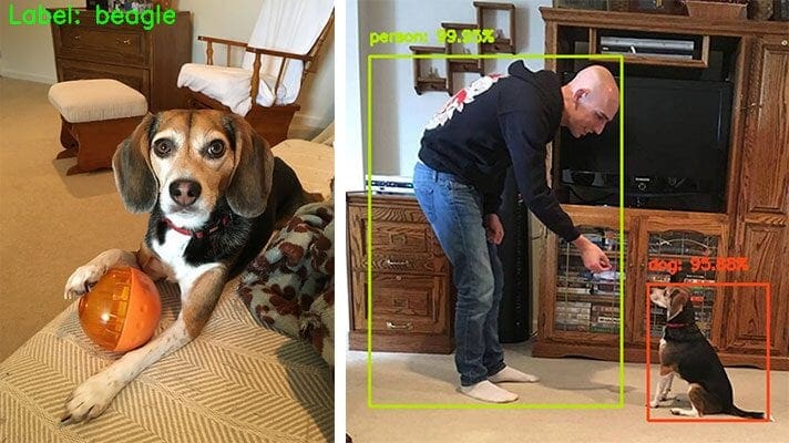
When performing image classification, given an input image, we present it to our neural network, and we obtain a single class label and a probability associated with the class label prediction (Figure 1, left).
This class label is meant to characterize the contents of the entire image, or at least the most dominant, visible contents of the image.
We can thus think of image classification as:
- One image in
- One class label out
Object detection, on the other hand, not only tells us what is in the image (i.e., class label) but also where in the image the object is via bounding box (x, y)-coordinates (Figure 1, right).
Therefore, object detection algorithms allow us to:
- Input one image
- Obtain multiple bounding boxes and class labels as output
At the very core, any object detection algorithm (regardless of traditional computer vision or state-of-the-art deep learning), follows the same pattern:
- 1. Input: An image that we wish to apply object detection to
- 2. Output: Three values, including:
- 2a. A list of bounding boxes, or the (x, y)-coordinates for each object in an image
- 2b. The class label associated with each of the bounding boxes
- 2c. The probability/confidence score associated with each bounding box and class label
Today, you’ll see an example of this pattern in action.
How can we turn any deep learning image classifier into an object detector?
At this point, you’re likely wondering:
Hey Adrian, if I have a Convolutional Neural Network trained for image classification, how in the world am I going to use it for object detection?
Based on your explanation above, it seems like image classification and object detection are fundamentally different, requiring two different types of network architectures.
And essentially, that is correct — object detection does require a specialized network architecture.
Anyone who has read papers on Faster R-CNN, Single Shot Detectors (SSDs), YOLO, RetinaNet, etc. knows that object detection networks are more complex, more involved, and take multiple orders of magnitude and more effort to implement compared to traditional image classification.
That said, there is a hack we can leverage to turn our CNN image classifier into an object detector — and the secret sauce lies in traditional computer vision algorithms.
Back before deep learning-based object detectors, the state-of-the-art was to use HOG + Linear SVM to detect objects in an image.
We’ll be borrowing elements from HOG + Linear SVM to convert any deep neural network image classifier into an object detector.
The first key ingredient from HOG + Linear SVM is to use image pyramids.
An “image pyramid” is a multi-scale representation of an image:
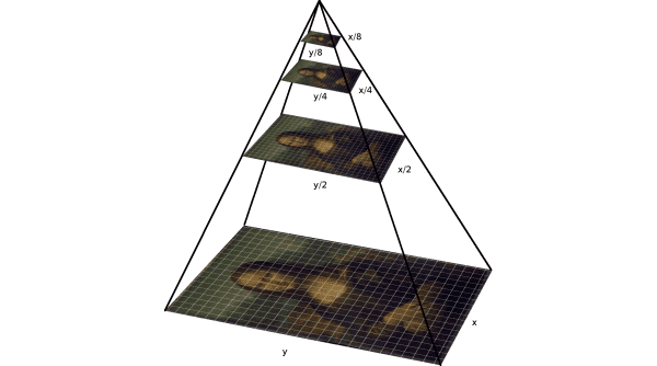
Utilizing an image pyramid allows us to find objects in images at different scales (i.e., sizes) of an image (Figure 2).
At the bottom of the pyramid, we have the original image at its original size (in terms of width and height).
And at each subsequent layer, the image is resized (subsampled) and optionally smoothed (usually via Gaussian blurring).
The image is progressively subsampled until some stopping criterion is met, which is normally when a minimum size has been reached and no further subsampling needs to take place.
The second key ingredient we need is sliding windows:
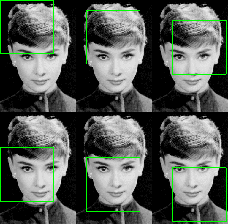
As the name suggests, a sliding window is a fixed-size rectangle that slides from left-to-right and top-to-bottom within an image. (As Figure 3 demonstrates, our sliding window could be used to detect the face in the input image).
At each stop of the window we would:
- Extract the ROI
- Pass it through our image classifier (ex., Linear SVM, CNN, etc.)
- Obtain the output predictions
Combined with image pyramids, sliding windows allow us to localize objects at different locations and multiple scales of the input image:
The final key ingredient we need is non-maxima suppression.
When performing object detection, our object detector will typically produce multiple, overlapping bounding boxes surrounding an object in an image.
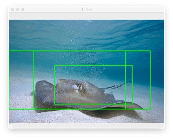
This behavior is totally normal — it simply implies that as the sliding window approaches an image, our classifier component is returning larger and larger probabilities of a positive detection.
Of course, multiple bounding boxes pose a problem — there’s only one object there, and we somehow need to collapse/remove the extraneous bounding boxes.
The solution to the problem is to apply non-maxima suppression (NMS), which collapses weak, overlapping bounding boxes in favor of the more confident ones:
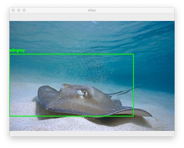
On the left, we have multiple detections, while on the right, we have the output of non-maxima suppression, which collapses the multiple bounding boxes into a single detection.
Combining traditional computer vision with deep learning to build an object detector
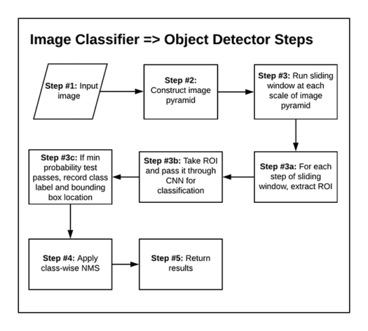
In order to take any Convolutional Neural Network trained for image classification and instead utilize it for object detection, we’re going to utilize the three key ingredients for traditional computer vision:
- Image pyramids: Localize objects at different scales/sizes.
- Sliding windows: Detect exactly where in the image a given object is.
- Non-maxima suppression: Collapse weak, overlapping bounding boxes.
The general flow of our algorithm will be:
- Step #1: Input an image
- Step #2: Construct an image pyramid
- Step #3: For each scale of the image pyramid, run a sliding window
- Step #3a: For each stop of the sliding window, extract the ROI
- Step #3b: Take the ROI and pass it through our CNN originally trained for image classification
- Step #3c: Examine the probability of the top class label of the CNN, and if meets a minimum confidence, record (1) the class label and (2) the location of the sliding window
- Step #4: Apply class-wise non-maxima suppression to the bounding boxes
- Step #5: Return results to calling function
That may seem like a complicated process, but as you’ll see in the remainder of this post, we can implement the entire object detection procedure in < 200 lines of code!
Configuring your development environment
To configure your system for this tutorial, I first recommend following either of these tutorials:
Either tutorial will help you configure your system with all the necessary software for this blog post in a convenient Python virtual environment.
Please note that PyImageSearch does not recommend or support Windows for CV/DL projects.
Project structure
Once you extract the .zip from the “Downloads” section of this blog post, your directory will be organized as follows:
.
├── images
│   ├── hummingbird.jpg
│   ├── lawn_mower.jpg
│   └── stingray.jpg
├── pyimagesearch
│   ├── __init__.py
│   └── detection_helpers.py
└── detect_with_classifier.py

2 directories, 6 files
Today’s pyimagesearch module contains a Python file — detection_helpers.py — consisting of two helper functions:
image_pyramid: Assists in generating copies of our image at different scales so that we can find objects of different sizessliding_window
Using the helper functions, our detect_with_classifier.py Python driver script accomplishes object detection by means of a classifier (using a sliding window and image pyramid approach). The classifier we’re using is a pre-trained ResNet50 CNN trained on the ImageNet dataset. The ImageNet dataset consists of 1,000 classes of objects.
Three images/ are provided for testing purposes. You should also test this script with images of your own — given that our classifier-based object detector can recognize 1,000 types of classes, most everyday objects and animals can be recognized. Have fun with it!
Implementing our image pyramid and sliding window utility functions
In order to turn our CNN image classifier into an object detector, we must first implement helper utilities to construct sliding windows and image pyramids.
Let’s implement this helper functions now — open up the detection_helpers.py file in the pyimagesearch module, and insert the following code:
# import the necessary packages
import imutils

def sliding_window(image, step, ws):
	# slide a window across the image
	for y in range(0, image.shape[0] - ws[1], step):
		for x in range(0, image.shape[1] - ws[0], step):
			# yield the current window
			yield (x, y, image[y:y + ws[1], x:x + ws[0]])
We begin by importing my package of convenience functions, imutils.
From there, we dive right in by defining our sliding_window generator function. This function expects three parameters:
image: The input image that we are going to loop over and generate windows from. This input image may come from the output of our image pyramid.step: Our step size, which indicates how many pixels we are going to “skip” in both the (x, y) directions. Normally, we would not want to loop over each and every pixel of the image (i.e.,step=1), as this would be computationally prohibitive if we were applying an image classifier at each window. Instead, the step size is determined on a per-dataset basis and is tuned to give optimal performance based on your dataset of images. In practice, it’s common to use astepof4to8pixels. Remember, the smaller your step size is, the more windows you’ll need to examine.ws: The window size defines the width and height (in pixels) of the window we are going to extract from ourimage. If you scroll back to Figure 3, the window size is equivalent to the dimensions of the green box that is sliding across the image.
The actual “sliding” of our window takes place on Lines 6-9 according to the following:
- Line 6 is our loop over our rows via determining a
rangeof y-values. - Line 7 is our loop over our columns (a
rangeof x-values). - Line 9 ultimately yields the window of our
image(i.e., ROI) according to the (x, y)-values, window size (ws), andstepsize.
The yield keyword is used in place of the return keyword because our sliding_window function is implemented as a Python generator.
For more information on our sliding windows implementation, please refer to my previous Sliding Windows for Object Detection with Python and OpenCV article.
Now that we’ve successfully defined our sliding window routine, let’s implement our image_pyramid generator used to construct a multi-scale representation of an input image:
def image_pyramid(image, scale=1.5, minSize=(224, 224)):
	# yield the original image
	yield image

	# keep looping over the image pyramid
	while True:
		# compute the dimensions of the next image in the pyramid
		w = int(image.shape[1] / scale)
		image = imutils.resize(image, width=w)

		# if the resized image does not meet the supplied minimum
		# size, then stop constructing the pyramid
		if image.shape[0] < minSize[1] or image.shape[1] < minSize[0]:
			break

		# yield the next image in the pyramid
		yield image
Our image_pyramid function accepts three parameters as well:
image: The input image for which we wish to generate multi-scale representations.scale: Our scale factor controls how much the image is resized at each layer. Smaller scale values yield more layers in the pyramid, and larger scale values yield fewer layers.minSizeminSizeparameter, ourwhileloop would continue forever (which is not what we want).
Now that we know the parameters that must be inputted to the function, let’s dive into the internals of our image pyramid generator function.
Referring to Figure 2, notice that the largest representation of our image is the input image itself. Line 13 of our generator simply yields the original, unaltered image the first time our generator is asked to produce a layer of our pyramid.
Subsequent generated images are controlled by the infinite while True loop beginning on Line 16.
Inside the loop, we first compute the dimensions of the next image in the pyramid according to our scale and the original image dimensions (Line 18). In this case, we simply divide the width of the input image by the scale to determine our width (w) ratio.
From there, we go ahead and resize the image down to the width while maintaining aspect ratio (Line 19). As you can see, we are using the aspect-aware resizing helper built into my imutils package.
While we are effectively done (we’ve resized our image, and now we can yield it), we need to implement an exit condition so that our generator knows to stop. As we learned when we defined our parameters to the image_pyramid function, the exit condition is determined by the minSize parameter. Therefore, the conditional on Lines 23 and 24 determines whether our resized image is too small (height or width) and exits the loop accordingly.
Assuming our scaled output image passes our minSize threshold, Line 27 yields it to the caller.
For more details, please refer to my Image Pyramids with Python and OpenCV article, which also includes an alternative scikit-image image pyramid implementation that may be useful to you.
Using Keras and TensorFlow to turn a pre-trained image classifier into an object detector
With our sliding_window and image_pyramid functions implemented, let’s now use them to take a deep neural network trained for image classification and turn it into an object detector.
Open up a new file, name it detect_with_classifier.py, and let’s begin coding:
# import the necessary packages
from tensorflow.keras.applications import ResNet50
from tensorflow.keras.applications.resnet import preprocess_input
from tensorflow.keras.preprocessing.image import img_to_array
from tensorflow.keras.applications import imagenet_utils
from imutils.object_detection import non_max_suppression
from pyimagesearch.detection_helpers import sliding_window
from pyimagesearch.detection_helpers import image_pyramid
import numpy as np
import argparse
import imutils
import time
import cv2
This script begins with a selection of imports including:
ResNet50: The popular ResNet Convolutional Neural Network (CNN) classifier by He et al. introduced in their 2015 paper, Deep Residual Learning for Image Recognition. We will load this CNN with pre-trained ImageNet weights.non_max_suppression: An implementation of NMS in my imutils package.sliding_window: Our sliding window generator function as described in the previous section.image_pyramid: The image pyramid generator that we defined previously.
Now that our imports are taken care of, let’s parse command line arguments:
# construct the argument parse and parse the arguments
ap = argparse.ArgumentParser()
ap.add_argument("-i", "--image", required=True,
	help="path to the input image")
ap.add_argument("-s", "--size", type=str, default="(200, 150)",
	help="ROI size (in pixels)")
ap.add_argument("-c", "--min-conf", type=float, default=0.9,
	help="minimum probability to filter weak detections")
ap.add_argument("-v", "--visualize", type=int, default=-1,
	help="whether or not to show extra visualizations for debugging")
args = vars(ap.parse_args())
The following arguments must be supplied to this Python script at runtime from your terminal:
--image--size--min-conf--visualize: A switch to determine whether to show additional visualizations for debugging.
We now have a handful of constants to define for our object detection procedures:
# initialize variables used for the object detection procedure
WIDTH = 600
PYR_SCALE = 1.5
WIN_STEP = 16
ROI_SIZE = eval(args["size"])
INPUT_SIZE = (224, 224)
Our classifier-based object detection methodology constants include:
WIDTHimages/for testing (refer to the “Project Structure” section) are all slightly different in size, we set a constant width here for later resizing purposes. By ensuring our images have a consistent starting width, we know that the image will fit on our screen.PYR_SCALE: Our image pyramid scale factor. This value controls how much the image is resized at each layer. Smaller scale values yield more layers in the pyramid, and larger scales yield fewer layers. The fewer layers you have, the faster the overall object detection system will operate, potentially at the expense of accuracy.WIN_STEP4and8to start with (depending on the dimensions of your input and yourminSize).ROI_SIZEminSizevalue — giving our image pyramid generator a means of exiting. As you can see, this value comes directly from our--sizecommand line argument.INPUT_SIZE: The classification CNN dimensions. Note that the tuple defined here on Line 32 heavily depends on the CNN you are using (in our case, it is ResNet50). If this notion doesn’t resonate with you, I suggest you read this tutorial and, more specifically the section entitled “Can I make the input dimensions [of a CNN] anything I want?”
Understanding what each of the above constants controls is crucial to your understanding of how to turn an image classifier into an object detector with Keras, TensorFlow, and OpenCV. Be sure to mentally distinguish each of these before moving on.
Let’s load our ResNet classification CNN and input image:
# load our network weights from disk
print("[INFO] loading network...")
model = ResNet50(weights="imagenet", include_top=True)

# load the input image from disk, resize it such that it has the
# has the supplied width, and then grab its dimensions
orig = cv2.imread(args["image"])
orig = imutils.resize(orig, width=WIDTH)
(H, W) = orig.shape[:2]
Line 36 loads ResNet pre-trained on ImageNet. If you choose to use a different pre-trained classifier, you can substitute one here for your particular project. To learn how to train your own classifier, I suggest you read Deep Learning for Computer Vision with Python.
We also load our input --image. Once it is loaded, we resize it (while maintaining aspect ratio according to our constant WIDTH) and grab resulting image dimensions.
From here, we’re ready to initialize our image pyramid generator object:
# initialize the image pyramid
pyramid = image_pyramid(orig, scale=PYR_SCALE, minSize=ROI_SIZE)

# initialize two lists, one to hold the ROIs generated from the image
# pyramid and sliding window, and another list used to store the
# (x, y)-coordinates of where the ROI was in the original image
rois = []
locs = []

# time how long it takes to loop over the image pyramid layers and
# sliding window locations
start = time.time()
On Line 45, we supply the necessary parameters to our image_pyramid generator function. Given that pyramid is a generator object at this point, we can loop over values it produces.
Before we do just that, Lines 50 and 51 initialize two lists:
rois: Holds the regions of interest (ROIs) generated from pyramid + sliding window outputlocs: Stores the (x, y)-coordinates of where the ROI was in the original image
And we also set a start timestamp so we can later determine how long our classification-based object detection method (given our parameters) took on the input image (Line 55).
Let’s loop over each image our pyramid produces:
# loop over the image pyramid
for image in pyramid:
	# determine the scale factor between the *original* image
	# dimensions and the *current* layer of the pyramid
	scale = W / float(image.shape[1])

	# for each layer of the image pyramid, loop over the sliding
	# window locations
	for (x, y, roiOrig) in sliding_window(image, WIN_STEP, ROI_SIZE):
		# scale the (x, y)-coordinates of the ROI with respect to the
		# *original* image dimensions
		x = int(x * scale)
		y = int(y * scale)
		w = int(ROI_SIZE[0] * scale)
		h = int(ROI_SIZE[1] * scale)

		# take the ROI and preprocess it so we can later classify
		# the region using Keras/TensorFlow
		roi = cv2.resize(roiOrig, INPUT_SIZE)
		roi = img_to_array(roi)
		roi = preprocess_input(roi)

		# update our list of ROIs and associated coordinates
		rois.append(roi)
		locs.append((x, y, x + w, y + h))
Looping over the layers of our image pyramid begins on Line 58.
Our first step in the loop is to compute the scale factor between the original image dimensions (W) and current layer dimensions (image.shape[1]) of our pyramid (Line 61). We need this value to later upscale our object bounding boxes.
Now we’ll cascade into our sliding window loop from this particular layer in our image pyramid. Our sliding_window generator allows us to look side-to-side and up-and-down in our image. For each ROI that it generates, we’ll soon apply image classification.
Line 65 defines our loop over our sliding windows. Inside, we:
- Scale coordinates (Lines 68-71).
- Grab the ROI and preprocess it (Lines 75-77). Preprocessing includes resizing to the CNN’s required
INPUT_SIZE, converting the image to array format, and applying Keras’ preprocessing convenience function. This includes adding a batch dimension, converting from RGB to BGR, and zero-centering color channels according to the ImageNet dataset. - Update the list of
roisand associatedlocscoordinates (Lines 80 and 81).
We also handle optional visualization:
		# check to see if we are visualizing each of the sliding
		# windows in the image pyramid
		if args["visualize"] > 0:
			# clone the original image and then draw a bounding box
			# surrounding the current region
			clone = orig.copy()
			cv2.rectangle(clone, (x, y), (x + w, y + h),
				(0, 255, 0), 2)

			# show the visualization and current ROI
			cv2.imshow("Visualization", clone)
			cv2.imshow("ROI", roiOrig)
			cv2.waitKey(0)
Here, we visualize both the original image with a green box indicating where we are “looking” and the resized ROI, which is ready for classification (Lines 85-95). As you can see, we’ll only --visualize when the flag is set via the command line.
Next, we’ll (1) check our benchmark on the pyramid + sliding window process, (2) classify all of our rois in batch, and (3) decode predictions:
# show how long it took to loop over the image pyramid layers and
# sliding window locations
end = time.time()
print("[INFO] looping over pyramid/windows took {:.5f} seconds".format(
	end - start))

# convert the ROIs to a NumPy array
rois = np.array(rois, dtype="float32")

# classify each of the proposal ROIs using ResNet and then show how
# long the classifications took
print("[INFO] classifying ROIs...")
start = time.time()
preds = model.predict(rois)
end = time.time()
print("[INFO] classifying ROIs took {:.5f} seconds".format(
	end - start))

# decode the predictions and initialize a dictionary which maps class
# labels (keys) to any ROIs associated with that label (values)
preds = imagenet_utils.decode_predictions(preds, top=1)
labels = {}
First, we end our pyramid + sliding window timer and show how long the process took (Lines 99-101).
Then, we take the ROIs and pass them (in batch) through our pre-trained image classifier (i.e., ResNet) via predict (Lines 104-118). As you can see, we print out a benchmark for the inference process here too.
Finally, Line 117 decodes the predictions, grabbing only the top prediction for each ROI.
We’ll need a means to map class labels (keys) to ROI locations associated with that label (values); the labels dictionary (Line 118) serves that purpose.
Let’s go ahead and populate our labels dictionary now:
# loop over the predictions
for (i, p) in enumerate(preds):
	# grab the prediction information for the current ROI
	(imagenetID, label, prob) = p[0]

	# filter out weak detections by ensuring the predicted probability
	# is greater than the minimum probability
	if prob >= args["min_conf"]:
		# grab the bounding box associated with the prediction and
		# convert the coordinates
		box = locs[i]

		# grab the list of predictions for the label and add the
		# bounding box and probability to the list
		L = labels.get(label, [])
		L.append((box, prob))
		labels[label] = L
Looping over predictions beginning on Line 121, we first grab the prediction information including the ImageNet ID, class label, and probability (Line 123).
From there, we check to see if the minimum confidence has been met (Line 127). Assuming so, we update the labels dictionary (Lines 130-136) with the bounding box and prob score tuple (value) associated with each class label (key).
As a recap, so far, we have:
- Generated scaled images with our image pyramid
- Generated ROIs using a sliding window approach for each layer (scaled image) of our image pyramid
- Performed classification on each ROI and placed the results in our
labelslist
We’re not quite done yet with turning our image classifier into an object detector with Keras, TensorFlow, and OpenCV. Now, we need to visualize the results.
This is the time where you would implement logic to do something useful with the results (labels), whereas in our case, we’re simply going to annotate the objects. We will also have to handle our overlapping detections by means of non-maxima suppression (NMS).
Let’s go ahead and loop over over all keys in our labels list:
# loop over the labels for each of detected objects in the image
for label in labels.keys():
	# clone the original image so that we can draw on it
	print("[INFO] showing results for '{}'".format(label))
	clone = orig.copy()

	# loop over all bounding boxes for the current label
	for (box, prob) in labels[label]:
		# draw the bounding box on the image
		(startX, startY, endX, endY) = box
		cv2.rectangle(clone, (startX, startY), (endX, endY),
			(0, 255, 0), 2)

	# show the results *before* applying non-maxima suppression, then
	# clone the image again so we can display the results *after*
	# applying non-maxima suppression
	cv2.imshow("Before", clone)
	clone = orig.copy()
Our loop over the labels for each of the detected objects begins on Line 139.
We make a copy of the original input image so that we can annotate it (Line 142).
We then annotate all bounding boxes for the current label (Lines 145-149).
So that we can visualize the before/after applying NMS, Line 154 displays the “before” image, and then we proceed to make another copy (Line 155).
Now, let’s apply NMS and display our “after” NMS visualization:
	# extract the bounding boxes and associated prediction
	# probabilities, then apply non-maxima suppression
	boxes = np.array([p[0] for p in labels[label]])
	proba = np.array([p[1] for p in labels[label]])
	boxes = non_max_suppression(boxes, proba)

	# loop over all bounding boxes that were kept after applying
	# non-maxima suppression
	for (startX, startY, endX, endY) in boxes:
		# draw the bounding box and label on the image
		cv2.rectangle(clone, (startX, startY), (endX, endY),
			(0, 255, 0), 2)
		y = startY - 10 if startY - 10 > 10 else startY + 10
		cv2.putText(clone, label, (startX, y),
			cv2.FONT_HERSHEY_SIMPLEX, 0.45, (0, 255, 0), 2)

	# show the output after apply non-maxima suppression
	cv2.imshow("After", clone)
	cv2.waitKey(0)
To apply NMS, we first extract the bounding boxes and associated prediction probabilities (proba) via Lines 159 and 160. We then pass those results into my imultils implementation of NMS (Line 161). For more details on non-maxima suppression, be sure to refer to my blog post.
After NMS has been applied, Lines 165-171 annotate bounding box rectangles and labels on the “after” image. Lines 174 and 175 display the results until a key is pressed, at which point all GUI windows close, and the script exits.
Great job! In the next section, we’ll analyze results of our method for using an image classifier for object detection purposes.
Image classifier to object detector results using Keras and TensorFlow
At this point, we are ready to see the results of our hard work.
Make sure you use the “Downloads” section of this tutorial to download the source code and example images from this blog post.
From there, open up a terminal, and execute the following command:
$ python detect_with_classifier.py --image images/stingray.jpg --size "(300, 150)"
[INFO] loading network...
[INFO] looping over pyramid/windows took 0.19142 seconds
[INFO] classifying ROIs...
[INFO] classifying ROIs took 9.67027 seconds
[INFO] showing results for 'stingray'
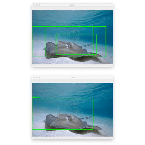
Here, you can see that I have inputted an example image containing a “stingray” which CNNs trained on ImageNet will be able to recognize (since ImageNet contains a “stingray” class).
Figure 7 (top) shows the original output from our object detection procedure.
Notice how there are multiple, overlapping bounding boxes surrounding the stingray.
Applying non-maxima suppression (Figure 7, bottom) collapses the bounding boxes into a single detection.
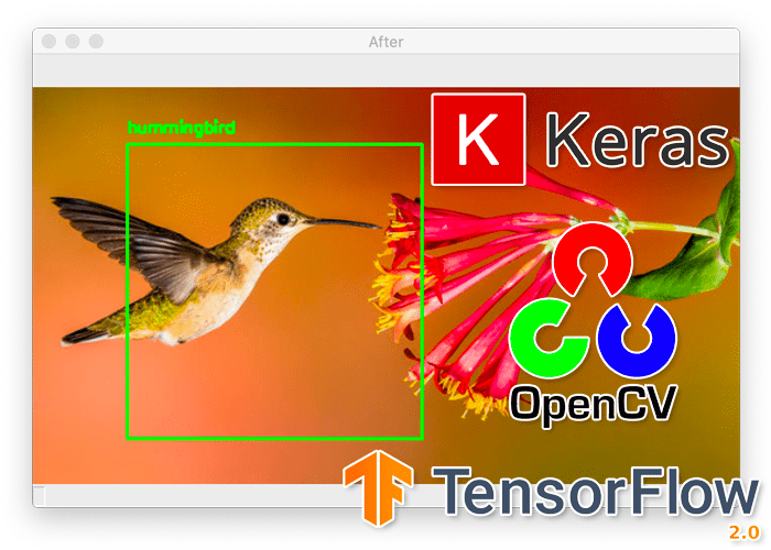
Let’s try another image, this one of a hummingbird (again, which networks trained on ImageNet will be able to recognize):
$ python detect_with_classifier.py --image images/hummingbird.jpg --size "(250, 250)"
[INFO] loading network...
[INFO] looping over pyramid/windows took 0.07845 seconds
[INFO] classifying ROIs...
[INFO] classifying ROIs took 4.07912 seconds
[INFO] showing results for 'hummingbird'
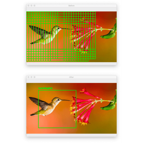
Figure 8 (top) shows the original output of our detection procedure, while the bottom shows the output after applying non-maxima suppression.
Again, our “image classifier turned object detector” procedure performed well here.
But let’s now try an example image where our object detection algorithm doesn’t perform optimally:
$ python detect_with_classifier.py --image images/lawn_mower.jpg --size "(200, 200)"
[INFO] loading network...
[INFO] looping over pyramid/windows took 0.13851 seconds
[INFO] classifying ROIs...
[INFO] classifying ROIs took 7.00178 seconds
[INFO] showing results for 'lawn_mower'
[INFO] showing results for 'half_track'

At first glance, it appears this method worked perfectly — we were able to localize the “lawn mower” in the input image.
But there was actually a second detection for a “half-track” (a military vehicle that has regular wheels on the front and tank-like tracks on the back):
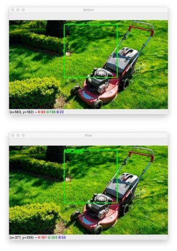
Clearly, there is not a half-track in this image, so how do we improve the results of our object detection procedure?
The answer is to increase our --min-conf to remove false-positive predictions:
$ python detect_with_classifier.py --image images/lawn_mower.jpg --size "(200, 200)" --min-conf 0.95
[INFO] loading network...
[INFO] looping over pyramid/windows took 0.13618 seconds
[INFO] classifying ROIs...
[INFO] classifying ROIs took 6.99953 seconds
[INFO] showing results for 'lawn_mower'
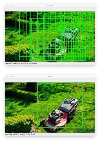
By increasing the minimum confidence to 95%, we have filtered out the less confident “half-track” prediction, leaving only the (correct) “lawn mower” object detection.
While our procedure for turning a pre-trained image classifier into an object detector isn’t perfect, it still can be used for certain situations, specifically when images are captured in controlled environments.
In the rest of this series, we’ll be learning how to improve upon our object detection results and build a more robust deep learning-based object detector.
Problems, limitations, and next steps
If you carefully inspect the results of our object detection procedure, you’ll notice a few key takeaways:
- The actual object detector is slow. Constructing all the image pyramid and sliding window locations takes ~1/10th of a second, and that doesn’t even include the time it takes for the network to make predictions on all the ROIs (4-9 seconds on a 3 GHz CPU)!
- Bounding box locations aren’t necessarily accurate. The largest issue with this object detection algorithm is that the accuracy of our detections is dependent on our selection of image pyramid scale, sliding window step, and ROI size. If any one of these values is off, then our detector is going to perform suboptimally.
- The network is not end-to-end trainable. The reason deep learning-based object detectors such as Faster R-CNN, SSDs, YOLO, etc. perform so well is because they are end-to-end trainable, meaning that any error in bounding box predictions can be made more accurate through backpropagation and updating the weights of the network — since we’re using a pre-trained image classifier with fixed weights, we cannot backpropagate error terms through the network.
Throughout this four-part series, we’ll be examining how to resolve these issues and build an object detector similar to the R-CNN family of networks.
What's next? We recommend PyImageSearch University.
86+ total classes • 115+ hours hours of on-demand code walkthrough videos • Last updated: March 2026
★★★★★ 4.84 (128 Ratings) • 16,000+ Students Enrolled
I strongly believe that if you had the right teacher you could master computer vision and deep learning.
Do you think learning computer vision and deep learning has to be time-consuming, overwhelming, and complicated? Or has to involve complex mathematics and equations? Or requires a degree in computer science?
That’s not the case.
All you need to master computer vision and deep learning is for someone to explain things to you in simple, intuitive terms. And that’s exactly what I do. My mission is to change education and how complex Artificial Intelligence topics are taught.
If you're serious about learning computer vision, your next stop should be PyImageSearch University, the most comprehensive computer vision, deep learning, and OpenCV course online today. Here you’ll learn how to successfully and confidently apply computer vision to your work, research, and projects. Join me in computer vision mastery.
Inside PyImageSearch University you'll find:
- ✓ 86+ courses on essential computer vision, deep learning, and OpenCV topics
- ✓ 86 Certificates of Completion
- ✓ 115+ hours hours of on-demand video
- ✓ Brand new courses released regularly, ensuring you can keep up with state-of-the-art techniques
- ✓ Pre-configured Jupyter Notebooks in Google Colab
- ✓ Run all code examples in your web browser — works on Windows, macOS, and Linux (no dev environment configuration required!)
- ✓ Access to centralized code repos for all 540+ tutorials on PyImageSearch
- ✓ Easy one-click downloads for code, datasets, pre-trained models, etc.
- ✓ Access on mobile, laptop, desktop, etc.
Summary
In this tutorial, you learned how to take any pre-trained deep learning image classifier and turn into an object detector using Keras, TensorFlow, and OpenCV.
To accomplish this task, we combined deep learning with traditional computer vision algorithms:
- In order to detect objects at different scales (i.e., sizes), we utilized image pyramids, which take our input image and repeatedly downsample it.
- To detect objects at different locations, we used sliding windows, which slide a fixed size window from left-to-right and top-to-bottom across the input image — at each stop of the window, we extract the ROI and pass it through our image classifier.
- It’s natural for object detection algorithms to produce multiple, overlapping bounding boxes for objects in an image; in order to “collapse” these overlapping bounding boxes into a single detection, we applied non-maxima suppression.
The end results of our hacked together object detection routine were fairly reasonable, but there were two primary problems:
- The network is not end-to-end trainable. We’re not actually “learning” to detect objects; we’re instead just taking ROIs and classifying them using a CNN trained for image classification.
- The object detection results are incredibly slow. On my Intel Xeon W 3 Ghz processor, applying object detection to a single image took ~4-9.5 seconds, depending on the input image resolution. Such an object detector could not be applied in real time.
In order to fix both of these problems, next week, we’ll start exploring the algorithms necessary to build an object detector from the R-CNN, Fast R-CNN, and Faster R-CNN family.
This will be a great series of tutorials, so you won’t want to miss them!
To download the source code to this post (and be notified when the next tutorial in this series publishes), simply enter your email address in the form below!

Download the Source Code and FREE 17-page Resource Guide
Enter your email address below to get a .zip of the code and a FREE 17-page Resource Guide on Computer Vision, OpenCV, and Deep Learning. Inside you'll find my hand-picked tutorials, books, courses, and libraries to help you master CV and DL!


Comment section
Hey, Adrian Rosebrock here, author and creator of PyImageSearch. While I love hearing from readers, a couple years ago I made the tough decision to no longer offer 1:1 help over blog post comments.
At the time I was receiving 200+ emails per day and another 100+ blog post comments. I simply did not have the time to moderate and respond to them all, and the sheer volume of requests was taking a toll on me.
Instead, my goal is to do the most good for the computer vision, deep learning, and OpenCV community at large by focusing my time on authoring high-quality blog posts, tutorials, and books/courses.
If you need help learning computer vision and deep learning, I suggest you refer to my full catalog of books and courses — they have helped tens of thousands of developers, students, and researchers just like yourself learn Computer Vision, Deep Learning, and OpenCV.
Click here to browse my full catalog.