Detect eyes, nose, lips, and jaw with dlib, OpenCV, and Python

Today’s blog post is part three in our current series on facial landmark detection and their applications to computer vision and image processing.

Two weeks ago I demonstrated how to install the dlib library which we are using for facial landmark detection.

Then, last week I discussed how to use dlib to actually detect facial landmarks in images.

Today we are going to take the next step and use our detected facial landmarks to help us label and extract face regions, including:

• Mouth
• Right eyebrow
• Left eyebrow
• Right eye
• Left eye
• Nose
• Jaw

To learn how to extract these face regions individually using dlib, OpenCV, and Python, just keep reading.

Detect eyes, nose, lips, and jaw with dlib, OpenCV, and Python

Today’s blog post will start with a discussion on the (x, y)-coordinates associated with facial landmarks and how these facial landmarks can be mapped to specific regions of the face.

We’ll then write a bit of code that can be used to extract each of the facial regions.

We’ll wrap up the blog post by demonstrating the results of our method on a few example images.

By the end of this blog post, you’ll have a strong understanding of how face regions are (automatically) extracted via facial landmarks and will be able to apply this knowledge to your own applications.

Facial landmark indexes for face regions

The facial landmark detector implemented inside dlib produces 68 (x, y)-coordinates that map to specific facial structures. These 68 point mappings were obtained by training a shape predictor on the labeled iBUG 300-W dataset.

Below we can visualize what each of these 68 coordinates map to:

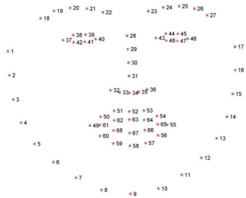
Examining the image, we can see that facial regions can be accessed via simple Python indexing (assuming zero-indexing with Python since the image above is one-indexed):

• The mouth can be accessed through points [48, 68].
• The right eyebrow through points [17, 22].
• The left eyebrow through points [22, 27].
• The right eye using [36, 42].
• The left eye with [42, 48].
• The nose using [27, 35].
• And the jaw via [0, 17].

These mappings are encoded inside the FACIAL_LANDMARKS_IDXS dictionary inside face_utils of the imutils library:

# define a dictionary that maps the indexes of the facial
# landmarks to specific face regions
FACIAL_LANDMARKS_IDXS = OrderedDict([
	("mouth", (48, 68)),
	("right_eyebrow", (17, 22)),
	("left_eyebrow", (22, 27)),
	("right_eye", (36, 42)),
	("left_eye", (42, 48)),
	("nose", (27, 35)),
	("jaw", (0, 17))
])

Using this dictionary we can easily extract the indexes into the facial landmarks array and extract various facial features simply by supplying a string as a key.

Visualizing facial landmarks with OpenCV and Python

A slightly harder task is to visualize each of these facial landmarks and overlay the results on an input image.

To accomplish this, we’ll need the visualize_facial_landmarks function, already included in the imutils library:

def visualize_facial_landmarks(image, shape, colors=None, alpha=0.75):
	# create two copies of the input image -- one for the
	# overlay and one for the final output image
	overlay = image.copy()
	output = image.copy()

	# if the colors list is None, initialize it with a unique
	# color for each facial landmark region
	if colors is None:
		colors = [(19, 199, 109), (79, 76, 240), (230, 159, 23),
			(168, 100, 168), (158, 163, 32),
			(163, 38, 32), (180, 42, 220)]

Our visualize_facial_landmarks function requires two arguments, followed by two optional ones, each detailed below:

• image : The image that we are going to draw our facial landmark visualizations on.
• shape : The NumPy array that contains the 68 facial landmark coordinates that map to various facial parts.
• colors : A list of BGR tuples used to color-code each of the facial landmark regions.
• alpha : A parameter used to control the opacity of the overlay on the original image.

Lines 45 and 46 create two copies of our input image — we’ll need these copies so that we can draw a semi-transparent overlay on the output image.

Line 50 makes a check to see if the colors list is None , and if so, initializes it with a preset list of BGR tuples (remember, OpenCV stores colors/pixel intensities in BGR order rather than RGB).

We are now ready to visualize each of the individual facial regions via facial landmarks:

	# loop over the facial landmark regions individually
	for (i, name) in enumerate(FACIAL_LANDMARKS_IDXS.keys()):
		# grab the (x, y)-coordinates associated with the
		# face landmark
		(j, k) = FACIAL_LANDMARKS_IDXS[name]
		pts = shape[j:k]

		# check if are supposed to draw the jawline
		if name == "jaw":
			# since the jawline is a non-enclosed facial region,
			# just draw lines between the (x, y)-coordinates
			for l in range(1, len(pts)):
				ptA = tuple(pts[l - 1])
				ptB = tuple(pts[l])
				cv2.line(overlay, ptA, ptB, colors[i], 2)

		# otherwise, compute the convex hull of the facial
		# landmark coordinates points and display it
		else:
			hull = cv2.convexHull(pts)
			cv2.drawContours(overlay, [hull], -1, colors[i], -1)

On Line 56 we loop over each entry in the FACIAL_LANDMARKS_IDXS dictionary.

For each of these regions, we extract the indexes of the given facial part and grab the (x, y)-coordinates from the shape NumPy array.

Lines 63-69 make a check to see if we are drawing the jaw, and if so, we simply loop over the individual points, drawing a line connecting the jaw points together.

Otherwise, Lines 73-75 handle computing the convex hull of the points and drawing the hull on the overlay.

The last step is to create a transparent overlay via the cv2.addWeighted function:

	# apply the transparent overlay
	cv2.addWeighted(overlay, alpha, output, 1 - alpha, 0, output)

	# return the output image
	return output

After applying visualize_facial_landmarks to an image and associated facial landmarks, the output would look similar to the image below:

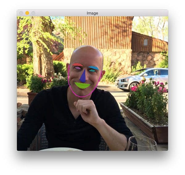
To learn how to glue all the pieces together (and extract each of these facial regions), let’s move on to the next section.

Extracting parts of the face using dlib, OpenCV, and Python

Before you continue with this tutorial, make sure you have:

1. Installed dlib according to my instructions in this blog post.
2. Have installed/upgraded imutils to the latest version, ensuring you have access to the face_utils submodule: pip install --upgrade imutils

From there, open up a new file, name it detect_face_parts.py , and insert the following code:

# import the necessary packages
from imutils import face_utils
import numpy as np
import argparse
import imutils
import dlib
import cv2

# construct the argument parser and parse the arguments
ap = argparse.ArgumentParser()
ap.add_argument("-p", "--shape-predictor", required=True,
	help="path to facial landmark predictor")
ap.add_argument("-i", "--image", required=True,
	help="path to input image")
args = vars(ap.parse_args())

# initialize dlib's face detector (HOG-based) and then create
# the facial landmark predictor
detector = dlib.get_frontal_face_detector()
predictor = dlib.shape_predictor(args["shape_predictor"])

# load the input image, resize it, and convert it to grayscale
image = cv2.imread(args["image"])
image = imutils.resize(image, width=500)
gray = cv2.cvtColor(image, cv2.COLOR_BGR2GRAY)

# detect faces in the grayscale image
rects = detector(gray, 1)

The first code block in this example is identical to the one in our previous tutorial.

We are simply:

• Importing our required Python packages (Lines 2-7).
• Parsing our command line arguments (Lines 10-15).
• Instantiating dlib’s HOG-based face detector and loading the facial landmark predictor (Lines 19 and 20).
• Loading and pre-processing our input image (Lines 23-25).
• Detecting faces in our input image (Line 28).

Again, for a more thorough, detailed overview of this code block, please see last week’s blog post on facial landmark detection with dlib, OpenCV, and Python.

Now that we have detected faces in the image, we can loop over each of the face ROIs individually:

# loop over the face detections
for (i, rect) in enumerate(rects):
	# determine the facial landmarks for the face region, then
	# convert the landmark (x, y)-coordinates to a NumPy array
	shape = predictor(gray, rect)
	shape = face_utils.shape_to_np(shape)

	# loop over the face parts individually
	for (name, (i, j)) in face_utils.FACIAL_LANDMARKS_IDXS.items():
		# clone the original image so we can draw on it, then
		# display the name of the face part on the image
		clone = image.copy()
		cv2.putText(clone, name, (10, 30), cv2.FONT_HERSHEY_SIMPLEX,
			0.7, (0, 0, 255), 2)

		# loop over the subset of facial landmarks, drawing the
		# specific face part
		for (x, y) in shape[i:j]:
			cv2.circle(clone, (x, y), 1, (0, 0, 255), -1)

For each face region, we determine the facial landmarks of the ROI and convert the 68 points into a NumPy array (Lines 34 and 35).

Then, for each of the face parts, we loop over them and on Line 38.

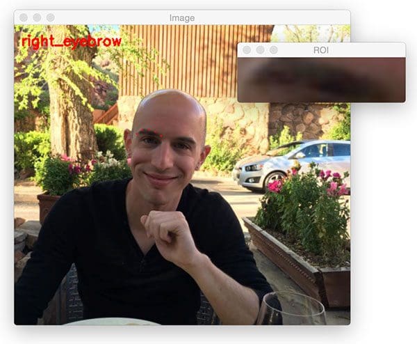
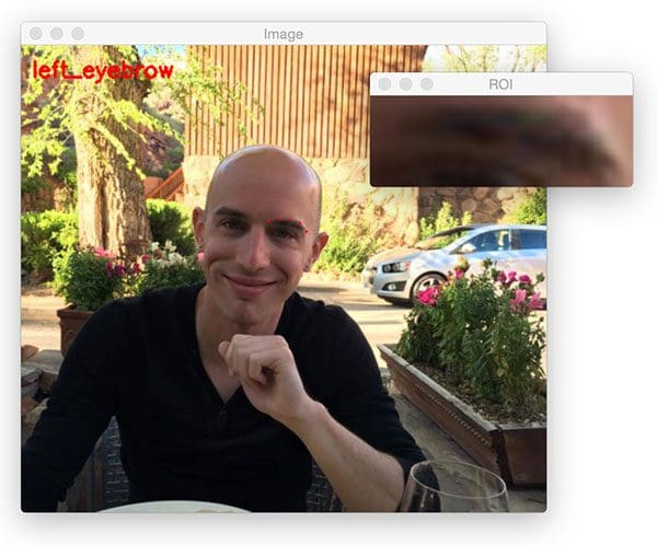
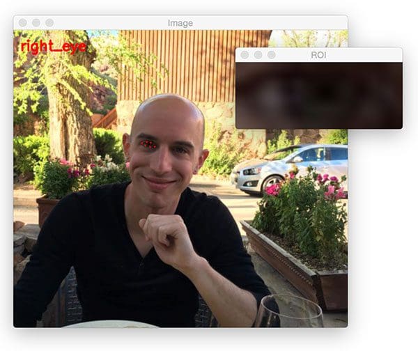
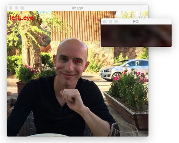
We draw the name/label of the face region on Lines 42 and 43, then draw each of the individual facial landmarks as circles on Lines 47 and 48.

To actually extract each of the facial regions we simply need to compute the bounding box of the (x, y)-coordinates associated with the specific region and use NumPy array slicing to extract it:

		# extract the ROI of the face region as a separate image
		(x, y, w, h) = cv2.boundingRect(np.array([shape[i:j]]))
		roi = image[y:y + h, x:x + w]
		roi = imutils.resize(roi, width=250, inter=cv2.INTER_CUBIC)

		# show the particular face part
		cv2.imshow("ROI", roi)
		cv2.imshow("Image", clone)
		cv2.waitKey(0)

	# visualize all facial landmarks with a transparent overlay
	output = face_utils.visualize_facial_landmarks(image, shape)
	cv2.imshow("Image", output)
	cv2.waitKey(0)

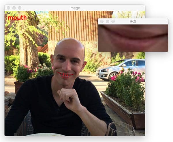
Computing the bounding box of the region is handled on Line 51 via cv2.boundingRect .

Using NumPy array slicing we can extract the ROI on Line 52.

This ROI is then resized to have a width of 250 pixels so we can better visualize it (Line 53).

Lines 56-58 display the individual face region to our screen.

Lines 61-63 then apply the visualize_facial_landmarks function to create a transparent overlay for each facial part.

Face part labeling results

Now that our example has been coded up, let’s take a look at some results.

Be sure to use the “Downloads” section of this guide to download the source code + example images + dlib facial landmark predictor model.

From there, you can use the following command to visualize the results:

$ python detect_face_parts.py --shape-predictor shape_predictor_68_face_landmarks.dat \
	--image images/example_01.jpg

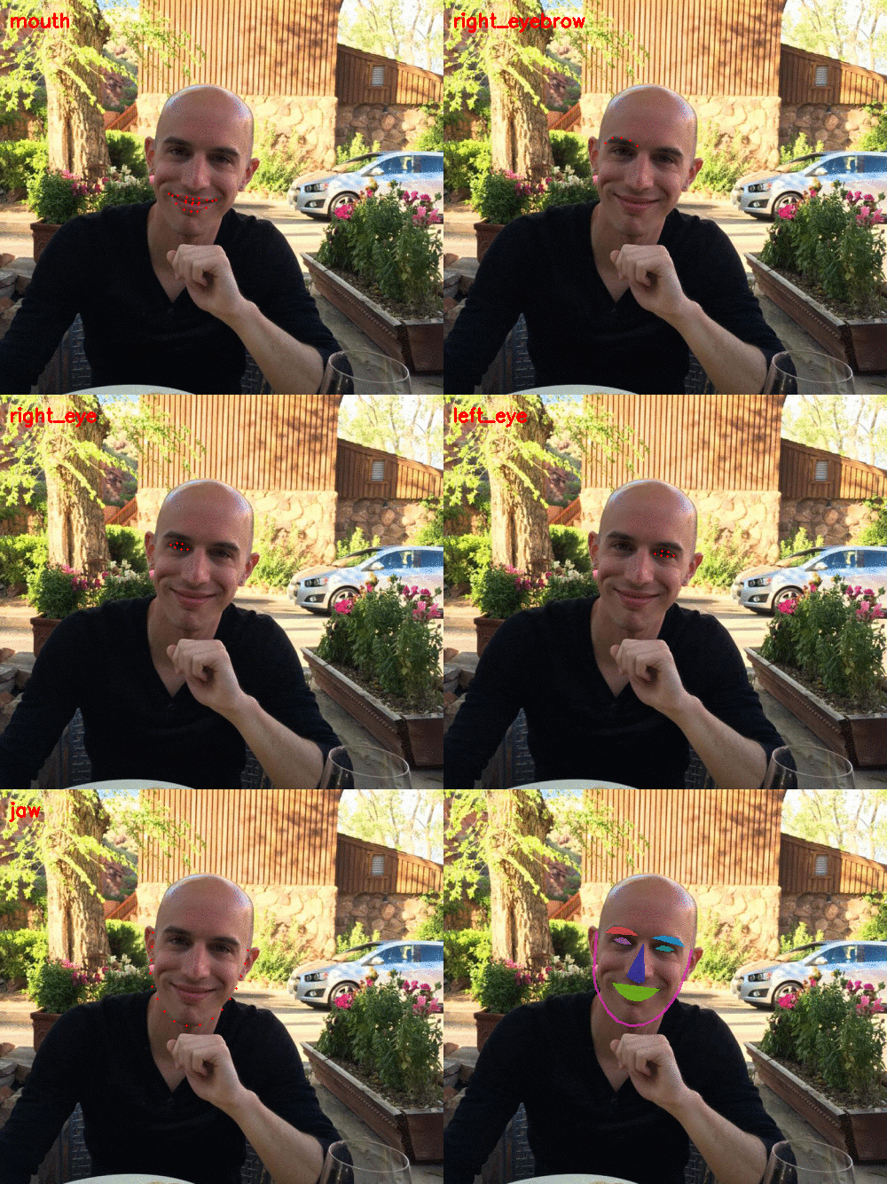
Notice how my mouth is detected first:

Followed by my right eyebrow:

Then the left eyebrow:

Next comes the right eye:

Along with the left eye:

And finally the jawline:

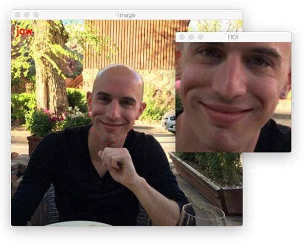
As you can see, the bounding box of the jawline is m entire face.

The last visualization for this image are our transparent overlays with each facial landmark region highlighted with a different color:

Let’s try another example:

$ python detect_face_parts.py --shape-predictor shape_predictor_68_face_landmarks.dat \
	--image images/example_02.jpg

This time I have created a GIF animation of the output:

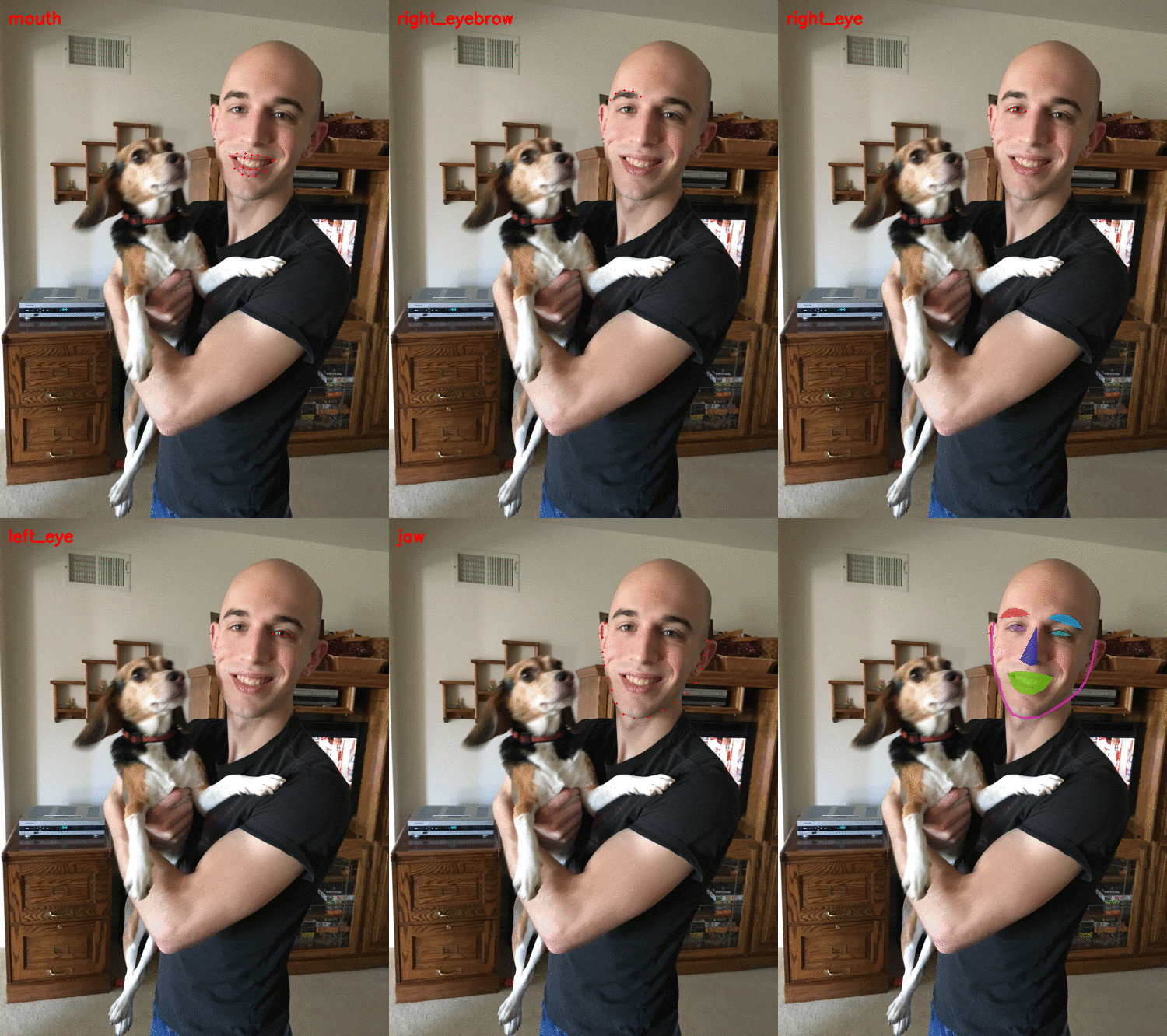
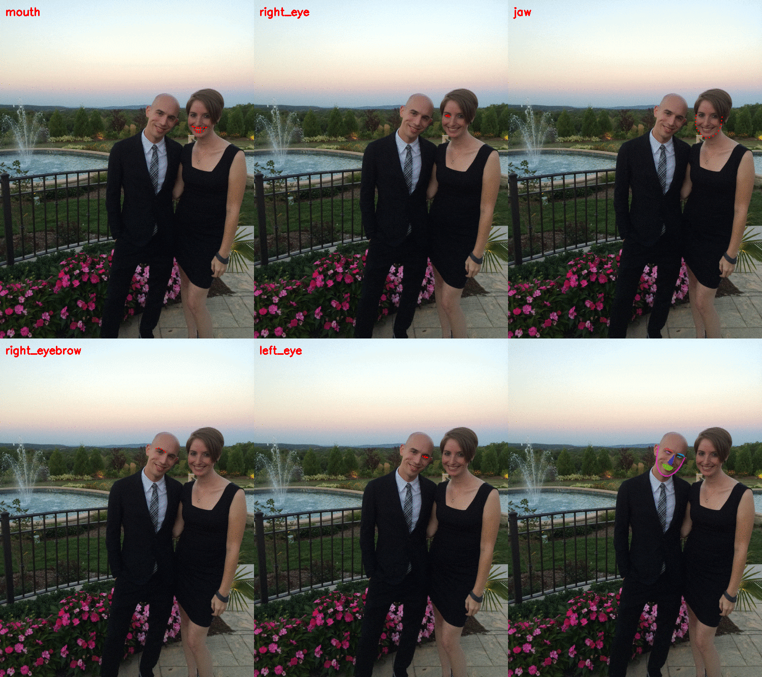
The same goes for our final example:

$ python detect_face_parts.py --shape-predictor shape_predictor_68_face_landmarks.dat \
	--image images/example_03.jpg

Summary

In this blog post I demonstrated how to detect various facial structures in an image using facial landmark detection.

Specifically, we learned how to detect and extract the:

• Mouth
• Right eyebrow
• Left eyebrow
• Right eye
• Left eye
• Nose
• Jawline

This was accomplished using dlib’s pre-trained facial landmark detector along with a bit of OpenCV and Python magic.

At this point you’re probably quite impressed with the accuracy of facial landmarks — and there are clear advantages of using facial landmarks, especially for face alignment, face swapping, and extracting various facial structures.

…but the big question is:

“Can facial landmark detection run in real-time?”

To find out, you’ll need to stay tuned for next week’s blog post.

To be notified when next week’s blog post on real-time facial landmark detection is published, be sure to enter your email address in the form below!

See you then.