Multi-class SVM Loss

A couple weeks ago,we discussed the concepts of both linear classification and parameterized learning. This type of learning allows us to take a set of input data and class labels, and actually learn a function that maps the input to the output predictions, simply by defining a set of parameters and optimizing over them.

Our linear classification tutorial focused mainly on the concept of a scoring function and how it can be used to map the input data to class labels. But in order to actually “learn” the mapping from the input data to class labels, we need to discuss two important concepts:

Loss functions
Optimization methods

In today and next week’s blog posts, we’ll be discussing two loss functions that you’ll commonly see when applying Machine Learning, Neural Networks, and Deep Learning algorithms:

Multi-class SVM loss
Cross-entropy (used for Softmax classifiers/Multinomial Logistic Regression)

To learn more about your first loss function, Multi-class SVM loss, just keep reading.

At the most basic level, a loss function is simply used to quantify how “good” or “bad” a given predictor is at classifying the input data points in a dataset.

The smaller the loss, the better a job our classifier is at modeling the relationship between the input data and the output class labels (although there is a point where we can overfit our model — this happens when the training data is modeled too closely and our model loses the ability to generalize).

Conversely, the larger our loss is, the more work needs to be done to increase classification accuracy. In terms of parameterized learning, this involves tuning parameters such as our weight matrix W or bias vector b to improve classification accuracy. Exactly how we go about updating these parameters is an optimization problem, which we’ll be covering later in this series of tutorials.

The mathematics behind Multi-class SVM loss

After reading through the linear classification with Python tutorial, you’ll note that we used a Linear Support Vector machine (SVM) as our classifier of choice.

This previous tutorial focused on the concept of a scoring function f that maps our feature vectors to class labels as numerical scores. As the name suggests, a Linear SVM applies a simple linear mapping:

$f(x_{i}, W, b) = Wx_{i} + b$

Now that we have this scoring/mapping function f, we need to determine how “good” or “bad” this function is (given the weight matrix W and bias vector b) at making predictions.

To accomplish this, we need a loss function. Let’s go ahead and start defining that now.

Based on our previous linear classification tutorial, we know that we have a matrix of feature vectors x — these feature vectors could be extracted color histograms, Histogram of Oriented Gradients features, or even raw pixel intensities.

Regardless of how we choose to quantify our images, the point is that we have a matrix x of features extracted from our image dataset. We can then access the features associated with a given image via the syntax $x_{i}$ , which will yield the i-th feature vector inside x.

Similarly, we also have a vector y which contains our class labels for each x. These y values are our ground-truth labels and what we hope our scoring function will correctly predict. Just like we can access a given feature vector via $x_{i}$ , we can access the i-th class label via $y_{i}$ .

As a matter of simplicity, let’s abbreviate our scoring function as s:

$s = f(x_{i}, W)$

Which implies that we can obtain the predicted score of the j-th class via for the i-th data point:

$s_{j} = f(x_{i}, W)_{j}$ .

Using this syntax, we can put it all together, obtaining the hinge loss function:

$L_{i} = \sum_{j \neq y_{i}} max(0, s_{j} - s_{y_{i}} + 1)$

Note: I’m purposely skipping the regularization parameter for now. We’ll return to regularization in a future post once we better understand loss functions.

So what is the above equation doing exactly?

I’m glad you asked.

Essentially, the hinge loss function is summing across all incorrect classes ( $i \neq j$ ) and comparing the output of our scoring function s returned for the j-th class label (the incorrect class) and the $y_{i}$ -th class (the correct class).

We apply the max operation to clamp values to 0 — this is important to do so that we do not end up summing negative values.

A given $x_{i}$ is classified correctly when the loss $L_{i} = 0$ (I’ll provide a numerical example of this in the following section).

To derive the loss across our entire training set, we simply take the mean over each individual $L_{i}$ :

$L = \frac{1}{N} \sum^{N}_{i=1} L_{i}$

Another related, common loss function you may come across is the squared hinge loss:

$L_{i} = \sum_{j \neq y_{i}} max(0, s_{j} - s_{y_{i}} + 1)^{2}$

The squared term penalizes our loss more heavily by squaring the output. This leads to a quadratic growth in loss rather than a linear one.

As for which loss function you should use, that is entirely dependent on your dataset. It’s typical to see the standard hinge loss function used more often, but on some datasets the squared variation might obtain better accuracy — overall, this is a hyperparameter that you should cross-validate.

A Multi-class SVM loss example

Now that we’ve taken a look at the mathematics behind hinge loss and squared hinge loss, let’s take a look at a worked example.

We’ll again assume that we’re working with the Kaggle Dogs vs. Cats dataset, which as the name suggests, aims to classify whether a given image contains a dog or a cat.

There are only two possible class labels in this dataset and is therefore a 2-class problem which can be solved using a standard, binary SVM loss function. That said, let’s still apply Multi-class SVM loss so we can have a worked example on how to apply it. From there, I’ll extend the example to handle a 3-class problem as well.

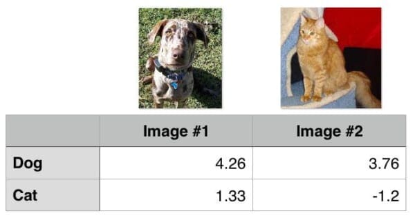
To start, take a look at the following figure where I have included 2 training examples from the 2 classes of the Dogs vs. Cats dataset:

Figure 1: Let's apply hinge loss to the images in this figure. — **Figure 1:** Let’s apply hinge loss to the images in this figure.

Given some (arbitrary) weight matrix W and bias vector b, the output scores of $f(x, W) = Wx + b$ are displayed in the body of the matrix. The larger the scores are, the more confident our scoring function is regarding the prediction.

Let’s start by computing the loss $L_{i}$ for the “dog” class. Given a two class problem, this is trivially easy:

>>> max(0, 1.33 - 4.26 + 1)
0
>>>

Notice how the loss for “dog” is zero — this implies that the dog class was correctly predicted. A quick investigation of Figure 1 above demonstrates this to be true: the “dog” score is greater than the “cat” score.

Similarly, we can do the same for the second image, this one containing a cat:

>>> max(0, 3.76 - (-1.2) + 1)
5.96
>>>

In this case, our loss function is greater than zero, indicating that our prediction is not correct.

We then obtain the total loss over the two example images by taking the average:

>>> (0 + 5.96) / 2
2.98
>>

That was simple enough for a 2-class problem, but what about a 3-class problem? Does the process become more complicated?

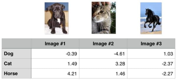
In reality, it doesn’t — our summation just expands a bit. You can find an example of a 3-class problem below, were I have added a third class, “horse”:

Figure 2: An example of applying hinge loss to a 3-class image classification problem. — **Figure 2:** An example of applying hinge loss to a 3-class image classification problem.

Let’s again compute the loss for the dog class:

>>> max(0, 1.49 - (-0.39) + 1) + max(0, 4.21 - (-0.39) + 1)
8.48
>>>

Notice how that our summation has expanded to include two terms — the difference between the predicted dog score and both the cat and horse score.

Similarly, we can compute the loss for the cat class:

>>> max(0, -4.61 - 3.28 + 1) + max(0, 1.46 - 3.28 + 1)
0
>>>

And finally the loss for the horse class:

>>> max(0, 1.03 - (-2.27) + 1) + max(0, -2.37 - (-2.27) + 1)
5.199999999999999
>>>

The total loss is therefore:

>>> (8.48 + 0.0 + 5.2) / 3
4.56
>>>

As you can see, the same general principles apply — just keep in mind that as the number of classes expands, your summation will expand as well.

Quiz: Based on the loss from the three classes above, which one was classified correctly?

Do I need to implement Multi-class SVM Loss by hand?

If you want, you could implement hinge loss and squared hinge loss by hand — but this would mainly be for educational purposes.

You’ll see both hinge loss and squared hinge loss implemented in nearly any machine learning/deep learning library, including scikit-learn, Keras, Caffe, etc.

What's next? We recommend PyImageSearch University.

Course information:
86 total classes • 115+ hours of on-demand code walkthrough videos • Last updated: October 2024
★★★★★ 4.84 (128 Ratings) • 16,000+ Students Enrolled

I strongly believe that if you had the right teacher you could master computer vision and deep learning.

Do you think learning computer vision and deep learning has to be time-consuming, overwhelming, and complicated? Or has to involve complex mathematics and equations? Or requires a degree in computer science?

That’s not the case.

All you need to master computer vision and deep learning is for someone to explain things to you in simple, intuitive terms. And that’s exactly what I do. My mission is to change education and how complex Artificial Intelligence topics are taught.

If you're serious about learning computer vision, your next stop should be PyImageSearch University, the most comprehensive computer vision, deep learning, and OpenCV course online today. Here you’ll learn how to successfully and confidently apply computer vision to your work, research, and projects. Join me in computer vision mastery.

Inside PyImageSearch University you'll find:

✓ 86 courses on essential computer vision, deep learning, and OpenCV topics
✓ 86 Certificates of Completion
✓ 115+ hours of on-demand video
✓ Brand new courses released regularly, ensuring you can keep up with state-of-the-art techniques
✓ Pre-configured Jupyter Notebooks in Google Colab
✓ Run all code examples in your web browser — works on Windows, macOS, and Linux (no dev environment configuration required!)
✓ Access to centralized code repos for all 540+ tutorials on PyImageSearch
✓ Easy one-click downloads for code, datasets, pre-trained models, etc.
✓ Access on mobile, laptop, desktop, etc.

Click here to join PyImageSearch University

Summary

Today I discussed the concept of Multi-class SVM loss. Given a scoring function (which maps input data to output class labels), our loss function can be used to quantify how “good” or “bad” our scoring function is at predicting the correct class labels in our dataset.

The smaller the loss, the more accurate our predictions are (but we also run the risk of “overfitting”, where we model the mapping of the input data to class labels too closely).

Conversely, the larger the loss, the less accurate our predictions are, thus we need to optimize our W and b parameters further — but we’ll save optimization methods for future posts once we better understand loss functions.

After understanding the concept of “loss” and how it applies to machine learning and deep learning algorithms, we then looked at two specific loss functions:

Hinge loss
Squared hinge loss

In general, you’l see hinge loss more often — but it’s still worth attempting to tune the hyperparameters to your classifier to determine which loss function gives better accuracy on your particular dataset.

Next week I’ll be back to discuss a second loss function — cross-entropy — and the relation it has to Multinomial Logistic Regression. If you have any prior experience in machine learning or deep learning, you may know this function better as the Softmax classifier.

If you’re interested in applying Deep Learning and Convolutional Neural Networks, then you don’t want to miss this upcoming post — as you’ll find out, the Softmax classifier is the most used model/loss function in Deep Learning.

To be notified when the next blog post is published, just enter your email address in the form below. See you next week!

Join the PyImageSearch Newsletter and Grab My FREE 17-page Resource Guide PDF

Enter your email address below to join the PyImageSearch Newsletter and download my FREE 17-page Resource Guide PDF on Computer Vision, OpenCV, and Deep Learning.