OpenCV Track Object Movement

This past Saturday, I was caught in the grips of childhood nostalgia, so I busted out my PlayStation 1 and my original copy of Final Fantasy VII. As a kid in late middle school/early high school, I logged 70+ hours playing through this heartbreaking, inspirational, absolute masterpiece of an RPG.

As a kid in middle school (when I had a lot more free time), this game was almost like a security blanket, a best friend, a make-believe world encoded in 1’s in 0’s where I could escape to, far away from the daily teenage angst, anxiety, and apprehension.

I spent so much time inside this alternate world that I completed nearly every single side quest. Ultimate and Ruby weapon? No problem. Omnislash? Done. Knights of the Round? Master level.

It probably goes without saying that Final Fantasy VII is my favorite RPG of all time — and it feels absolutely awesome to be playing it again.

But as I sat on my couch a couple nights ago, sipping a seasonal Sam Adams Octoberfest while entertaining my old friends Cloud, Tifa, Barret, and the rest of the gang, it got me thinking: “Not only have video games evolved dramatically over the past 10 years, but the controllers have as well.”

Think about it. While it a bit gimmicky, the Wii Remote was a major paradigm shift in user/game interaction. Over on the PlayStation side, we had PlayStation Move, essentially a wand with both (1) an internal motion sensors, (2) and an external motion tracking component via a webcam hooked up to the PlayStation 3 itself. Of course, then there is the XBox Kinect (one of the largest modern day computer vision success stories, especially within the gaming area) that required no extra remote or wand — using a stereo camera and a regression forest for pose classification, the Kinect allowed you to become the controller.

This week’s blog post is an extension to last week’s tutorial on ball tracking with OpenCV. We won’t be learning how to build the next generation, groundbreaking video game controller — but I will show you how to track object movement in images, allowing you to determine the direction an object is moving:

Read on to learn more.

Looking for the source code to this post?

Jump Right To The Downloads Section

OpenCV Track Object Movement

Note: The code for this post is heavily based on last’s weeks tutorial on ball tracking with OpenCV, so because of this I’ll be shortening up a few code reviews. If you want more detail for a given code snippet, please refer to the original blog post on ball tracking.

Let’s go ahead and get started. Open up a new file, name it object_movement.py , and we’ll get to work:

# import the necessary packages
from collections import deque
from imutils.video import VideoStream
import numpy as np
import argparse
import cv2
import imutils
import time

# construct the argument parse and parse the arguments
ap = argparse.ArgumentParser()
ap.add_argument("-v", "--video",
	help="path to the (optional) video file")
ap.add_argument("-b", "--buffer", type=int, default=32,
	help="max buffer size")
args = vars(ap.parse_args())

We start off by importing our necessary packages on Lines 2-8. We need Python’s built in deque datatype to efficiently store the past N points the object has been detected and tracked at. We’ll also need imutils, by collection of OpenCV and Python convenience functions. If you’re a follower of this blog, you likely already have this package installed. If you don’t have imutils installed/upgraded yet, let pip take care of the installation process:

$ pip install --upgrade imutils

Lines 11-16 handle parsing our two (optional) command line arguments. If you want to use a video file with this example script, just pass the path to the video file to the object_movement.py script using the --video switch. If the --video switch is omitted, your webcam will (attempted) to be used instead.

We also have a second command line argument, --buffer , which controls the maximum size of the deque of points. The larger the deque the more (x, y)-coordinates of the object are tracked, essentially giving you a larger “history” of where the object has been in the video stream. We’ll default the --buffer to be 32, indicating that we’ll maintain a buffer of (x, y)-coordinates of our object for only the previous 32 frames.

Now that we have our packages imported and our command line arguments parsed, let’s continue on:

# define the lower and upper boundaries of the "green"
# ball in the HSV color space
greenLower = (29, 86, 6)
greenUpper = (64, 255, 255)

# initialize the list of tracked points, the frame counter,
# and the coordinate deltas
pts = deque(maxlen=args["buffer"])
counter = 0
(dX, dY) = (0, 0)
direction = ""

# if a video path was not supplied, grab the reference
# to the webcam
if not args.get("video", False):
	vs = VideoStream(src=0).start()

# otherwise, grab a reference to the video file
else:
	vs = cv2.VideoCapture(args["video"])

# allow the camera or video file to warm up
time.sleep(2.0)

Lines 20 and 21 define the lower and upper boundaries of the color green in the HSV color space (since we will be tracking the location of a green ball in our video stream). Let’s also initialize our pts variable to be a deque with a maximum size of buffer (Line 25).

From there, Lines 25-28 initialize a few bookkeeping variables we’ll utilize to compute and display the actual direction the ball is moving in the video stream.

Lastly, Lines 32-37 handle grabbing a pointer, vs , to either our webcam or video file. We are taking advantage of the imutils.video VideoStream class to handle the camera frames in a threaded approach. To handle the video file, cv2.VideoCapture does the best job.

Now that we have a pointer to our video stream we can start looping over the individual frames and processing them one-by-one:

# keep looping
while True:
	# grab the current frame
	frame = vs.read()

	# handle the frame from VideoCapture or VideoStream
	frame = frame[1] if args.get("video", False) else frame

	# if we are viewing a video and we did not grab a frame,
	# then we have reached the end of the video
	if frame is None:
		break

	# resize the frame, blur it, and convert it to the HSV
	# color space
	frame = imutils.resize(frame, width=600)
	blurred = cv2.GaussianBlur(frame, (11, 11), 0)
	hsv = cv2.cvtColor(blurred, cv2.COLOR_BGR2HSV)

	# construct a mask for the color "green", then perform
	# a series of dilations and erosions to remove any small
	# blobs left in the mask
	mask = cv2.inRange(hsv, greenLower, greenUpper)
	mask = cv2.erode(mask, None, iterations=2)
	mask = cv2.dilate(mask, None, iterations=2)

	# find contours in the mask and initialize the current
	# (x, y) center of the ball
	cnts = cv2.findContours(mask.copy(), cv2.RETR_EXTERNAL,
		cv2.CHAIN_APPROX_SIMPLE)
	cnts = imutils.grab_contours(cnts)
	center = None

This snippet of code is identical to last week’s post on ball tracking so please refer to that post for more detail, but the gist is:

• Line 43: Start looping over the frames from the vs pointer (whether that’s a video file or a webcam stream).
• Line 45: Grab the next frame from the video stream. Line 48 takes care of parsing either a tuple or variable directly.
• Lines 52 and 53: If a frame could not not be read, break from the loop.
• Lines 57-59: Pre-process the frame by resizing it, applying a Gaussian blur to smooth the image and reduce high frequency noise, and finally convert the frame to the HSV color space.
• Lines 64-66: Here is where the “green color detection” takes place. A call to cv2.inRange using the greenLower and greenUpper boundaries in the HSV color space leaves us with a binary mask representing where in the image the color “green” is found. A series of erosions and dilations are applied to remove small blobs in the mask .

You can see an example of the binary mask below:

On the left we have our original frame and on the right we can clearly see that only the green ball has been detected, while all other background and foreground objects are filtered out.

Finally, we use the cv2.findContours function to find the contours (i.e. “outlines”) of the objects in the binary mask (Lines 70-72).

Let’s find the ball contour:

	# only proceed if at least one contour was found
	if len(cnts) > 0:
		# find the largest contour in the mask, then use
		# it to compute the minimum enclosing circle and
		# centroid
		c = max(cnts, key=cv2.contourArea)
		((x, y), radius) = cv2.minEnclosingCircle(c)
		M = cv2.moments(c)
		center = (int(M["m10"] / M["m00"]), int(M["m01"] / M["m00"]))

		# only proceed if the radius meets a minimum size
		if radius > 10:
			# draw the circle and centroid on the frame,
			# then update the list of tracked points
			cv2.circle(frame, (int(x), int(y)), int(radius),
				(0, 255, 255), 2)
			cv2.circle(frame, center, 5, (0, 0, 255), -1)
			pts.appendleft(center)

This code is also near-identical to the previous post on ball tracking, but I’ll give a quick rundown of the code to ensure you understand what is going on:

• Line 76: Here we just make a quick check to ensure at least one object was found in our frame .
• Lines 80-83: Provided that at least one object (in this case, our green ball) was found, we find the largest contour (based on its area), and compute the minimum enclosing circle and the centroid of the object. The centroid is simply the center (x, y)-coordinates of the object.
• Lines 86-92: We’ll require that our object have at least a 10 pixel radius to track it — if it does, we’ll draw the minimum enclosing circle surrounding the object, draw the centroid, and finally update the list of pts containing the center (x, y)-coordinates of the object.

Unlike last weeks example that simply drew the contrail of the object as it moved around the frame, let’s see how we can actually track the object movement, followed by using this object movement to compute the direction the object is moving using only (x, y)-coordinates of the object:

	# loop over the set of tracked points
	for i in np.arange(1, len(pts)):
		# if either of the tracked points are None, ignore
		# them
		if pts[i - 1] is None or pts[i] is None:
			continue

		# check to see if enough points have been accumulated in
		# the buffer
		if counter >= 10 and i == 1 and pts[-10] is not None:
			# compute the difference between the x and y
			# coordinates and re-initialize the direction
			# text variables
			dX = pts[-10][0] - pts[i][0]
			dY = pts[-10][1] - pts[i][1]
			(dirX, dirY) = ("", "")

			# ensure there is significant movement in the
			# x-direction
			if np.abs(dX) > 20:
				dirX = "East" if np.sign(dX) == 1 else "West"

			# ensure there is significant movement in the
			# y-direction
			if np.abs(dY) > 20:
				dirY = "North" if np.sign(dY) == 1 else "South"

			# handle when both directions are non-empty
			if dirX != "" and dirY != "":
				direction = "{}-{}".format(dirY, dirX)

			# otherwise, only one direction is non-empty
			else:
				direction = dirX if dirX != "" else dirY

On Line 95 we start to loop over the (x, y)-coordinates of object we are tracking. If either of the points are None (Lines 98 and 99) we simply ignore them and keep looping.

Otherwise, we can actually compute the direction the object is moving by investigating two previous (x, y)-coordinates.

Computing the directional movement (if any) is handled on Lines 107 and 108 where we compute dX and dY , the deltas (differences) between the x and y coordinates of the current frame and a frame towards the end of the buffer, respectively.

However, it’s important to note that there is a bit of a catch to performing this computation. An obvious first solution would be to compute the direction of the object between the current frame and the previous frame. However, using the current frame and the previous frame is a bit of an unstable solution. Unless the object is moving very quickly, the deltas between the (x, y)-coordinates will be very small. If we were to use these deltas to report direction, then our results would be extremely noisy, implying that even small, minuscule changes in trajectory would be considered a direction change. In fact, these changes could be so small that they would be near invisible to the human eye (or at the very least, trivial) — we are most likely not that interested reporting and tracking such small movements.

Instead, it’s much more likely that we are interested in the larger object movements and reporting the direction in which the object is moving — hence we compute the deltas between the coordinates of the current frame and a frame farther back in the queue. Performing this operation helps reduce noise and false reports of direction change.

On Line 113 we check the magnitude of the x-delta to see if there is a significant difference in direction along the x-axis. In this case, if there is more than 20 pixel difference between the x-coordinates, we need to figure out in which direction the object is moving. If the sign of dX is positive, then we know the object is moving to the right (east). Otherwise, if the sign of dX is negative, then we are moving to the left (west).

Note: You can make the direction detection code more sensitive by decreasing the threshold. In this case, a 20 pixel different obtains good results. However, if you want to detect tiny movements, simply decrease this value. On the other hand, if you want to only report large object movements, all you need to do is increase this threshold.

Lines 118 and 119 handle dY in a similar fashion. First, we must ensure there is a significant change in movement (at least 20 pixels). If so, we can check the sign of dY . If the sign of dY is positive, then we’re moving up (north), otherwise the sign is negative and we’re moving down (south).

However, it could be the case that both dX and dY have substantial directional movements (indicating diagonal movement, such as “South-East” or “North-West”). Lines 122 and 123 handle the case our object is moving along a diagonal and update the direction variable as such.

At this point, our script is pretty much done! We just need to wrap a few more things up:

		# otherwise, compute the thickness of the line and
		# draw the connecting lines
		thickness = int(np.sqrt(args["buffer"] / float(i + 1)) * 2.5)
		cv2.line(frame, pts[i - 1], pts[i], (0, 0, 255), thickness)

	# show the movement deltas and the direction of movement on
	# the frame
	cv2.putText(frame, direction, (10, 30), cv2.FONT_HERSHEY_SIMPLEX,
		0.65, (0, 0, 255), 3)
	cv2.putText(frame, "dx: {}, dy: {}".format(dX, dY),
		(10, frame.shape[0] - 10), cv2.FONT_HERSHEY_SIMPLEX,
		0.35, (0, 0, 255), 1)

	# show the frame to our screen and increment the frame counter
	cv2.imshow("Frame", frame)
	key = cv2.waitKey(1) & 0xFF
	counter += 1

	# if the 'q' key is pressed, stop the loop
	if key == ord("q"):
		break

# if we are not using a video file, stop the camera video stream
if not args.get("video", False):
	vs.stop()

# otherwise, release the camera
else:
	vs.release()

# close all windows
cv2.destroyAllWindows()

Again, this code is essentially identical to the previous post on ball tracking, so I’ll just give a quick rundown:

• Lines 131 and 132: Here we compute the thickness of the contrail of the object and draw it on our frame .
• Lines 138-140: This code handles drawing some diagnostic information to our frame , such as the direction in which the object is moving along with the dX and dY deltas used to derive the direction , respectively.
• Lines 143-149: Display the frame to our screen and wait for a keypress. If the q key is pressed, we’ll break from the while loop on Line 149.
• Lines 152-160: Cleanup our vs pointer and close any open windows.

Testing out our object movement tracker

Now that we have coded up a Python and OpenCV script to track object movement, let’s give it a try. Fire up a shell and execute the following command:

$ python object_movement.py --video object_tracking_example.mp4

Below we can see an animation of the OpenCV tracking object movement script:

However, let’s take a second to examine a few of the individual frames.

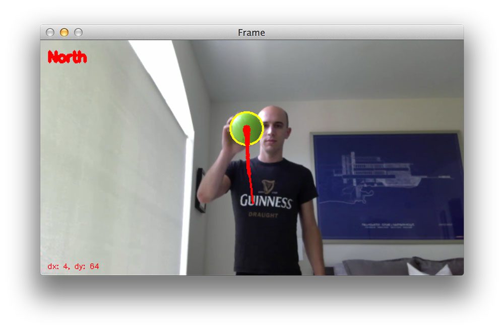
From the above figure we can see that the green ball has been successfully detected and is moving north. The “north” direction was determined by examining the dX and dY values (which are displayed at the bottom-left of the frame). Since |dY| > 20 we were able to determine there was a significant change in y-coordinates. The sign of dY is also positive, allowing us to determine the direction of movement is north.

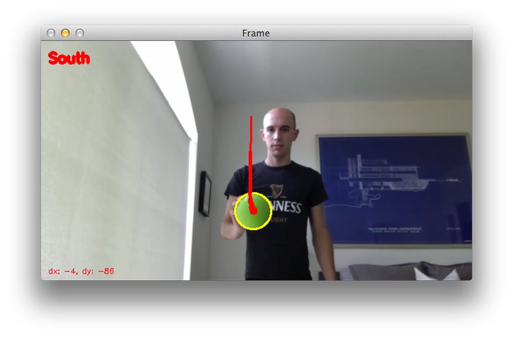
Again, |dY| > 20, but this time the sign is negative, so we must be moving south.

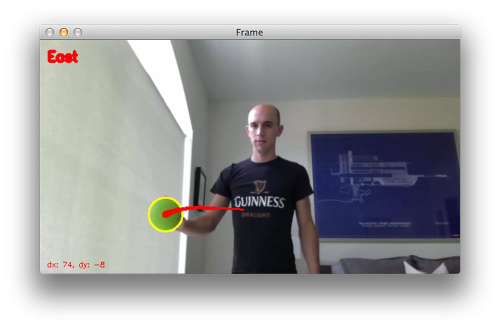
In the above image we can see that the ball is moving east. It may appear that the ball is moving west (to the left); however, keep in mind that our viewpoint is reversed, so my right is actually your left.

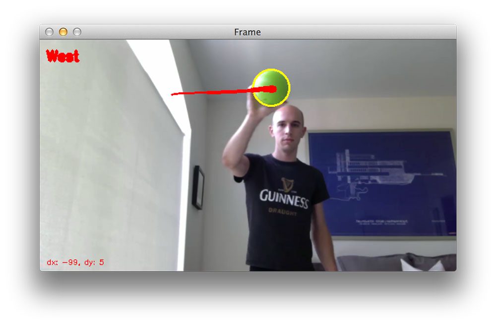
Just as we can track movements to the east, we can also track movements to the west.

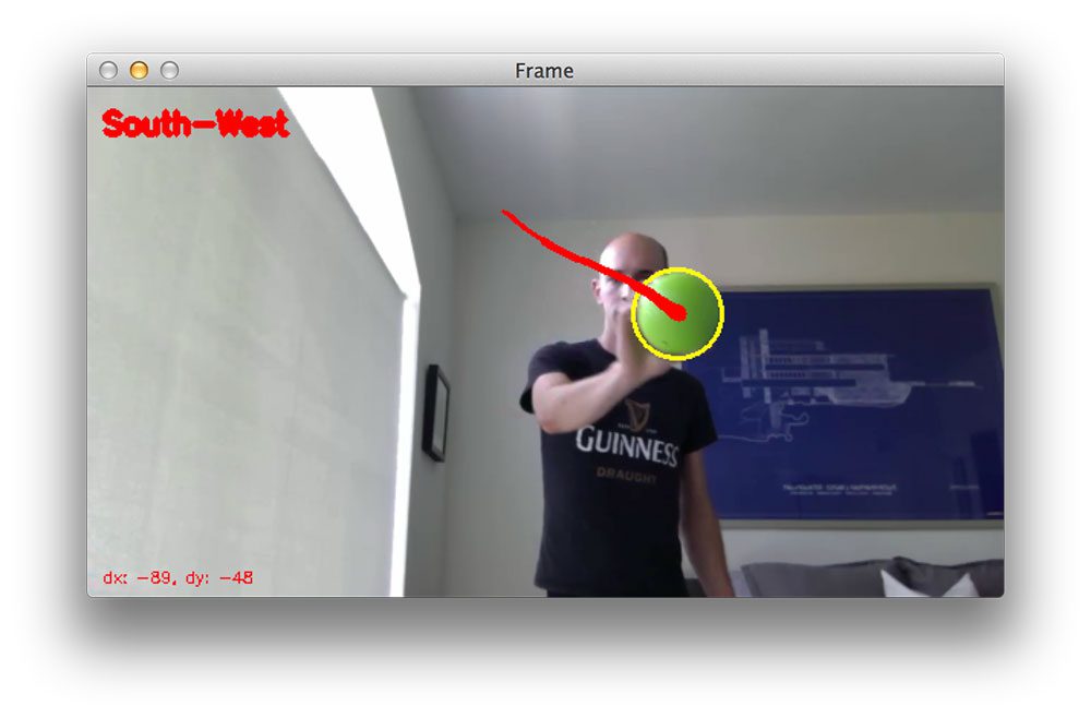
Moving across a diagonal is also not an issue. When both |dX| > 20 and |dY| > 20, we know that the ball is moving across a diagonal.

You can see the full demo video here:

If you want the object_movement.py script to access your webcam stream rather than the supplied object_tracking_example.mp4 video supplied in the code download of this post, simply omit the --video switch:

$ python object_movement.py

What's next? We recommend PyImageSearch University.

Course information:
86+ total classes • 115+ hours hours of on-demand code walkthrough videos • Last updated: October 2025
★★★★★ 4.84 (128 Ratings) • 16,000+ Students Enrolled

I strongly believe that if you had the right teacher you could master computer vision and deep learning.

Do you think learning computer vision and deep learning has to be time-consuming, overwhelming, and complicated? Or has to involve complex mathematics and equations? Or requires a degree in computer science?

That’s not the case.

All you need to master computer vision and deep learning is for someone to explain things to you in simple, intuitive terms. And that’s exactly what I do. My mission is to change education and how complex Artificial Intelligence topics are taught.

If you're serious about learning computer vision, your next stop should be PyImageSearch University, the most comprehensive computer vision, deep learning, and OpenCV course online today. Here you’ll learn how to successfully and confidently apply computer vision to your work, research, and projects. Join me in computer vision mastery.

Inside PyImageSearch University you'll find:

• ✓ 86+ courses on essential computer vision, deep learning, and OpenCV topics
• ✓ 86 Certificates of Completion
• ✓ 115+ hours hours of on-demand video
• ✓ Brand new courses released regularly, ensuring you can keep up with state-of-the-art techniques
• ✓ Pre-configured Jupyter Notebooks in Google Colab
• ✓ Run all code examples in your web browser — works on Windows, macOS, and Linux (no dev environment configuration required!)
• ✓ Access to centralized code repos for all 540+ tutorials on PyImageSearch
• ✓ Easy one-click downloads for code, datasets, pre-trained models, etc.
• ✓ Access on mobile, laptop, desktop, etc.

Click here to join PyImageSearch University

Summary

In this blog post you learned about tracking object direction (not to mention, my childhood obsession with Final Fantasy VII).

This tutorial started as an extension to our previous article on ball tracking. While the ball tracking tutorial showed us the basics of object detection and tracking, we were unable to compute the actual direction the ball was moving. By simply computing the deltas between (x, y)-coordinates of the object in two separate frames, we were able to correctly track object movement and even report the direction it was moving.

We could make this object movement tracker even more precise by reporting the actual angle of movement simply by taking the arctangent of dX  and dY  respectively — but I’ll leave that as an exercise to you, the reader.

Be sure to download the code to this post and give it a try!

Download the Source Code and FREE 17-page Resource Guide

Enter your email address below to get a .zip of the code and a FREE 17-page Resource Guide on Computer Vision, OpenCV, and Deep Learning. Inside you'll find my hand-picked tutorials, books, courses, and libraries to help you master CV and DL!

Download the code!

Website