Let’s face it. Trying to search for images based on text and tags sucks.
Whether you are tagging and categorizing your personal images, searching for stock photos for your company website, or simply trying to find the right image for your next epic blog post, trying to use text and keywords to describe something that is inherently visual is a real pain.
I faced this pain myself last Tuesday as I was going through some old family photo albums there were scanned and digitized nine years ago.
You see, I was looking for a bunch of photos that were taken along the beaches of Hawaii with my family. I opened up iPhoto, and slowly made my way through the photographs. It was a painstaking process. The meta-information for each JPEG contained incorrect dates. The photos were not organized in folders like I remembered — I simply couldn’t find the beach photos that I was desperately searching for.
Perhaps by luck, I stumbled across one of the beach photographs. It was a beautiful, almost surreal beach shot. Puffy white clouds in the sky. Crystal clear ocean water, lapping at the golden sands. You could literally feel the breeze on your skin and smell the ocean air.
After seeing this photo, I stopped my manual search and opened up a code editor.
While applications such as iPhoto let you organize your photos into collections and even detect and recognize faces, we can certainly do more.
No, I’m not talking about manually tagging your images. I’m talking about something more powerful. What if you could actually search your collection of images using an another image?
Wouldn’t that be cool? It would allow you to apply visual search to your own images, in just a single click.
And that’s exactly what I did. I spent the next half-hour coding and when I was done I had created a visual search engine for my family vacation photos.
I then took the sole beach image that I found and then submitted it to my image search engine. Within seconds I had found all of the other beach photos, all without labeling or tagging a single image.
Sound interesting? Read on.
In the rest of this blog post I’ll show you how to build an image search engine of your own.
What’s an Image Search Engine?
So you’re probably wondering, what actually is an image search engine?
I mean, we’re all familiar with text based search engines such as Google, Bing, and DuckDuckGo — you simply enter a few keywords related to the content you want to find (i.e., your “query”), and then your results are returned to you. But for image search engines, things work a little differently — you’re not using text as your query, you are instead using an image.
Sounds pretty hard to do, right? I mean, how do you quantify the contents of an image to make it search-able?
We’ll cover the answer to that question in a bit. But to start, let’s learn a little more about image search engines.
In general, there tend to be three types of image search engines: search by meta-data, search by example, and a hybrid approach of the two.
Search by Meta-Data
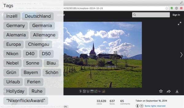
Searching by meta-data is only marginally different than your standard keyword-based search engines mentioned above. Search by meta-data systems rarely examine the contents of the image itself. Instead, they rely on textual clues such as (1) manual annotations and tagging performed by humans along with (2) automated contextual hints, such as the text that appears near the image on a webpage.
When a user performs a search on a search by meta-data system they provide a query, just like in a traditional text search engine, and then images that have similar tags or annotations are returned.
Again, when utilizing a search by meta-data system the actual image itself is rarely examined.
A great example of a Search by Meta-Data image search engine is Flickr. After uploading an image to Flickr you are presented with a text field to enter tags describing the contents of images you have uploaded. Flickr then takes these keywords, indexes them, and utilizes them to find and recommend other relevant images.
Search by Example
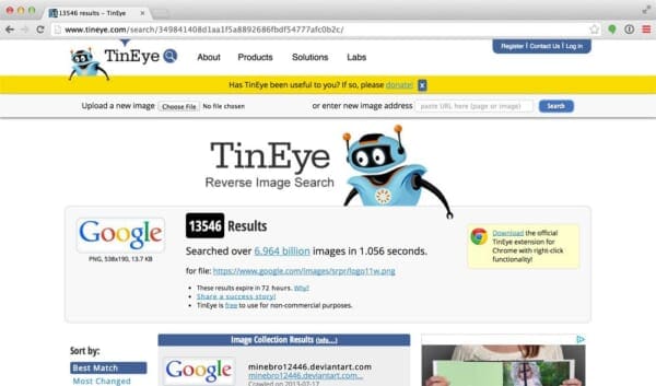
Search by example systems, on the other hand, rely solely on the contents of the image — no keywords are assumed to be provided. The image is analyzed, quantified, and stored so that similar images are returned by the system during a search.
Image search engines that quantify the contents of an image are called Content-Based Image Retrieval (CBIR) systems. The term CBIR is commonly used in the academic literature, but in reality, it’s simply a fancier way of saying “image search engine”, with the added poignancy that the search engine is relying strictly on the contents of the image and not any textual annotations associated with the image.
A great example of a Search by Example system is TinEye. TinEye is actually a reverse image search engine where you provide a query image, and then TinEye returns near-identical matches of the same image, along with the webpage that the original image appeared on.
Take a look at the example image at the top of this section. Here I have uploaded an image of the Google logo. TinEye has examined the contents of the image and returned to me the 13,000+ webpages that the Google logo appears on after searching through an index of over 6 billion images.
So consider this: Are you going to manually label each of these 6 billion images in TinEye? Of course not. That would take an army of employees and would be extremely costly.
Instead, you utilize some sort of algorithm to extract “features” (i.e., a list of numbers to quantify and abstractly represent the image) from the image itself. Then, when a user submits a query image, you extract features from the query image and compare them to your database of features and try to find similar images.
Again, it’s important to reinforce the point that Search by Example systems rely strictly on the contents of the image. These types of systems tend to be extremely hard to build and scale, but allow for a fully automated algorithm to govern the search — no human intervention is required.
Hybrid Approach
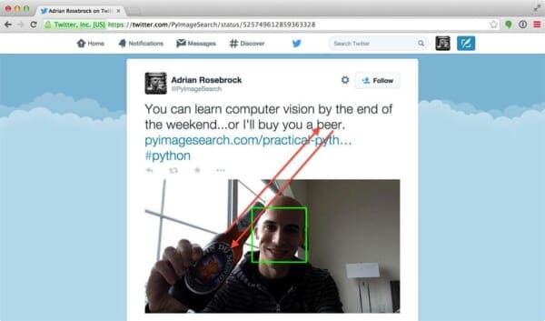
Of course, there is a middle ground between the two – consider Twitter, for instance.
On Twitter you can upload photos to accompany your tweets. A hybrid approach would be to correlate the features extracted from the image with the text of the tweet. Using this approach you could build an image search engine that could take both contextual hints along with a Search by Example strategy.
Note: Interested in reading more about the different types of image search engines? I have an entire blog post dedicated to comparing and contrasting them, available here.
Let’s move on to defining some important terms that we’ll use regularly when describing and building image search engines.
Some Important Terms
Before we get too in-depth, let’s take a little bit of time to define a few important terms.
When building an image search engine we will first have to index our dataset. Indexing a dataset is the process of quantifying our dataset by utilizing an image descriptor to extract features from each image.
An image descriptor defines the algorithm that we are utilizing to describe our image.
For example:
- The mean and standard deviation of each Red, Green, and Blue channel, respectively,
- The statistical moments of the image to characterize shape.
- The gradient magnitude and orientation to describe both shape and texture.
The important takeaway here is that the image descriptor governs how the image is quantified.
Features, on the other hand, are the output of an image descriptor. When you put an image into an image descriptor, you will get features out the other end.
In the most basic terms, features (or feature vectors) are just a list of numbers used to abstractly represent and quantify images.
Take a look at the example figure below:

Here we are presented with an input image, we apply our image descriptor, and then our output is a list of features used to quantify the image.
Feature vectors can then be compared for similarity by using a distance metric or similarity function. Distance metrics and similarity functions take two feature vectors as inputs and then output a number that represents how “similar” the two feature vectors are.
The figure below visualizes the process of comparing two images:
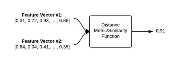
Given two feature vectors, a distance function is used to determine how similar the two feature vectors are. The output of the distance function is a single floating point value used to represent the similarity between the two images.
The 4 Steps of Any CBIR System
No matter what Content-Based Image Retrieval System you are building, they all can be boiled down into 4 distinct steps:
- Defining your image descriptor: At this phase you need to decide what aspect of the image you want to describe. Are you interested in the color of the image? The shape of an object in the image? Or do you want to characterize texture?
- Indexing your dataset: Now that you have your image descriptor defined, your job is to apply this image descriptor to each image in your dataset, extract features from these images, and write the features to storage (ex. CSV file, RDBMS, Redis, etc.) so that they can be later compared for similarity.
- Defining your similarity metric: Cool, now you have a bunch of feature vectors. But how are you going to compare them? Popular choices include the Euclidean distance, Cosine distance, and chi-squared distance, but the actual choice is highly dependent on (1) your dataset and (2) the types of features you extracted.
- Searching: The final step is to perform an actual search. A user will submit a query image to your system (from an upload form or via a mobile app, for instance) and your job will be to (1) extract features from this query image and then (2) apply your similarity function to compare the query features to the features already indexed. From there, you simply return the most relevant results according to your similarity function.
Again, these are the most basic 4 steps of any CBIR system. As they become more complex and utilize different feature representations, the number of steps grow and you’ll add a substantial number of sub-steps to each step mentioned above. But for the time being, let’s keep things simple and utilize just these 4 steps.
Let’s take a look at a few graphics to make these high-level steps a little more concrete. The figure below details Steps 1 and 2:

We start by taking our dataset of images, extracting features from each image, and then storing these features in a database.
We can then move on to performing a search (Steps 3 and 4):
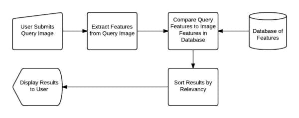
First, a user must submit a query image to our image search engine. We then take the query image and extract features from it. These “query features” are then compared to the features of the images we already indexed in our dataset. Finally, the results are then sorted by relevancy and presented to the user.
Our Dataset of Vacation Photos
We’ll be utilizing the INRIA Holidays Dataset for our dataset of images.
This dataset consists of various vacation trips from all over the world, including photos of the Egyptian pyramids, underwater diving with sea-life, forests in the mountains, wine bottles and plates of food at dinner, boating excursions, and sunsets across the ocean.
Here are a few samples from the dataset:
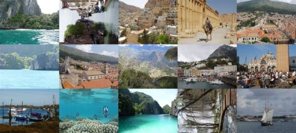
In general, this dataset does an extremely good job at modeling what we would expect a tourist to photograph on a scenic trip.
The Goal
Our goal here is to build a personal image search engine. Given our dataset of vacation photos, we want to make this dataset “search-able” by creating a “more like this” functionality — this will be a “search by example” image search engine. For instance, if I submit a photo of sail boats gliding across a river, our image search engine should be able to find and retrieve our vacation photos of when we toured the marina and docks.
Take a look at the example below where I have submitted an photo of the boats on the water and have found relevant images in our vacation photo collection:
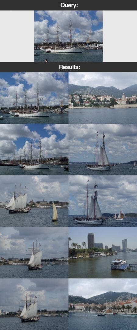
In order to build this system, we’ll be using a simple, yet effective image descriptor: the color histogram.
By utilizing a color histogram as our image descriptor, we’ll be we’ll be relying on the color distribution of the image. Because of this, we have to make an important assumption regarding our image search engine:
Assumption: Images that have similar color distributions will be considered relevant to each other. Even if images have dramatically different contents, they will still be considered “similar” provided that their color distributions are similar as well.
This is a really important assumption, but is normally a fair and reasonable assumption to make when using color histograms as image descriptors.
Step 1: Defining our Image Descriptor
Instead of using a standard color histogram, we are going to apply a few tricks and make it a little more robust and powerful.
Our image descriptor will be a 3D color histogram in the HSV color space (Hue, Saturation, Value). Typically, images are represented as a 3-tuple of Red, Green, and Blue (RGB). We often think of the RGB color space as “cube”, as shown below:
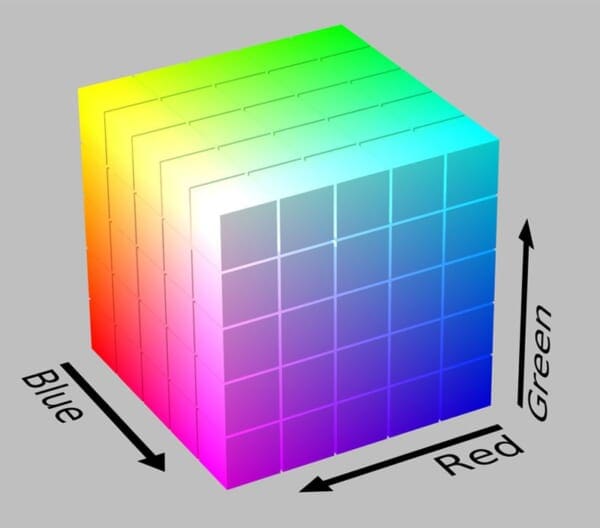
However, while RGB values are simple to understand, the RGB color space fails to mimic how humans perceive color. Instead, we are going to use the HSV color space which maps pixel intensities into a cylinder:
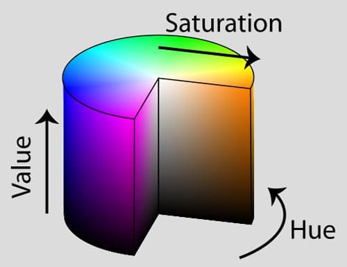
There are other color spaces that do an even better job at mimicking how humans perceive color, such as the CIE L*a*b* and CIE XYZ spaces, but let’s keep our color model relatively simple for our first image search engine implementation.
So now that we have selected a color space, we now need to define the number of bins for our histogram. Histograms are used to give a (rough) sense of the density of pixel intensities in an image. Essentially, our histogram will estimate the probability density of the underlying function, or in this case, the probability P of a pixel color C occurring in our image I.
It’s important to note that there is a trade-off with the number of bins you select for your histogram. If you select too few bins, then your histogram will have less components and unable to disambiguate between images with substantially different color distributions. Likewise, if you use too many bins your histogram will have many components and images with very similar contents may be regarded and “not similar” when in reality they are.
Here’s an example of a histogram with only a few bins:

Notice how there are very few bins that a pixel can be placed into.
And here’s an example of a histogram with lots of bins:
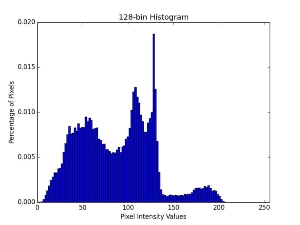
In the above example you can see that many bins are utilized, but with the larger number of bins, you lose your ability to “generalize” between images with similar perceptual content since all of the peaks and valleys of the histogram will have to match in order for two images to be considered “similar”.
Personally, I like an iterative, experimental approach to tuning the number of bins. This iterative approach is normally based on the size of my dataset. The more smaller that my dataset is, the less bins I use. And if my dataset is large, I use more bins, making my histograms larger and more discriminative.
In general, you’ll want to experiment with the number of bins for your color histogram descriptor as it is dependent on (1) the size of your dataset and (2) how similar the color distributions in your dataset are to each other.
For our vacation photo image search engine, we’ll be utilizing a 3D color histogram in the HSV color space with 8 bins for the Hue channel, 12 bins for the saturation channel, and 3 bins for the value channel, yielding a total feature vector of dimension 8 x 12 x 3 = 288.
This means that for every image in our dataset, no matter if the image is 36 x 36 pixels or 2000 x 1800 pixels, all images will be abstractly represented and quantified using only a list of 288 floating point numbers.
I think the best way to explain a 3D histogram is to use the conjunctive AND. A 3D HSV color descriptor will ask a given image how many pixels have a Hue value that fall into bin #1 AND how many pixels have a Saturation value that fall into bin #1 AND how many pixels have a Value intensity that fall into bin #1. The number of pixels that meet these requirements are then tabulated. This process is repeated for each combination of bins; however, we are able to do it in an extremely computationally efficient manner.
Pretty cool, right?
Anyway, enough talk. Let’s get into some code.
Open up a new file in your favorite code editor, name it colordescriptor.py and let’s get started:
# import the necessary packages
import numpy as np
import cv2
import imutils

class ColorDescriptor:
	def __init__(self, bins):
		# store the number of bins for the 3D histogram
		self.bins = bins

	def describe(self, image):
		# convert the image to the HSV color space and initialize
		# the features used to quantify the image
		image = cv2.cvtColor(image, cv2.COLOR_BGR2HSV)
		features = []

		# grab the dimensions and compute the center of the image
		(h, w) = image.shape[:2]
		(cX, cY) = (int(w * 0.5), int(h * 0.5))
We’ll start by importing the Python packages we’ll need. We’ll use NumPy for numerical processing, cv2 for our OpenCV bindings, and imutils to check OpenCV version.
We then define our ColorDescriptor class on Line 6. This class will encapsulate all the necessary logic to extract our 3D HSV color histogram from our images.
The __init__ method of the ColorDescriptor takes only a single argument, bins , which is the number of bins for our color histogram.
We can then define our describe method on Line 11. This method requires an image , which is the image we want to describe.
Inside of our describe method we’ll convert from the RGB color space (or rather, the BGR color space; OpenCV represents RGB images as NumPy arrays, but in reverse order) to the HSV color space, followed by initializing our list of features to quantify and represent our image .
Lines 18 and 19 simply grab the dimensions of the image and compute the center (x, y) coordinates.
So now the hard work starts.
Instead of computing a 3D HSV color histogram for the entire image, let’s instead compute a 3D HSV color histogram for different regions of the image.
Using regions-based histograms rather than global-histograms allows us to simulate locality in a color distribution. For example, take a look at this image below:
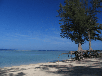
In this photo we can clearly see a blue sky at the top of the image and a sandy beach at the bottom. Using a global histogram we would be unable to determine where in the image the “blue” occurs and where the “brown” sand occurs. Instead, we would just know that there exists some percentage of blue and some percentage of brown.
To remedy this problem, we can compute color histograms in regions of the image:
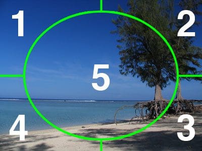
For our image descriptor, we are going to divide our image into five different regions: (1) the top-left corner, (2) the top-right corner, (3) the bottom-right corner, (4) the bottom-left corner, and finally (5) the center of the image.
By utilizing these regions we’ll be able to mimic a crude form of localization, being able to represent our above beach image as having shades of blue sky in the top-left and top-right corners, brown sand in the bottom-left and bottom-right corners, and then a combination of blue sky and brown sand in the center region.
That all said, here is the code to create our region-based color descriptor:
		# divide the image into four rectangles/segments (top-left,
		# top-right, bottom-right, bottom-left)
		segments = [(0, cX, 0, cY), (cX, w, 0, cY), (cX, w, cY, h),
			(0, cX, cY, h)]

		# construct an elliptical mask representing the center of the
		# image
		(axesX, axesY) = (int(w * 0.75) // 2, int(h * 0.75) // 2)
		ellipMask = np.zeros(image.shape[:2], dtype = "uint8")
		cv2.ellipse(ellipMask, (cX, cY), (axesX, axesY), 0, 0, 360, 255, -1)

		# loop over the segments
		for (startX, endX, startY, endY) in segments:
			# construct a mask for each corner of the image, subtracting
			# the elliptical center from it
			cornerMask = np.zeros(image.shape[:2], dtype = "uint8")
			cv2.rectangle(cornerMask, (startX, startY), (endX, endY), 255, -1)
			cornerMask = cv2.subtract(cornerMask, ellipMask)

			# extract a color histogram from the image, then update the
			# feature vector
			hist = self.histogram(image, cornerMask)
			features.extend(hist)

		# extract a color histogram from the elliptical region and
		# update the feature vector
		hist = self.histogram(image, ellipMask)
		features.extend(hist)

		# return the feature vector
		return features
Lines 23 and 24 start by defining the indexes of our top-left, top-right, bottom-right, and bottom-left regions, respectively.
From there, we’ll need to construct an ellipse to represent the center region of the image. We’ll do this by defining an ellipse radius that is 75% of the width and height of the image on Line 28.
We then initialize a blank image (filled with zeros to represent a black background) with the same dimensions of the image we want to describe on Line 29.
Finally, let’s draw the actual ellipse on Line 30 using the cv2.ellipse function. This function requires eight different parameters:
ellipMask: The image we want to draw the ellipse on. We’ll be using a concept of “masks” which I’ll discuss shortly.(cX, cY): A 2-tuple representing the center (x, y)-coordinates of the image.(axesX, axesY): A 2-tuple representing the length of the axes of the ellipse. In this case, the ellipse will stretch to be 75% of the width and height of theimagethat we are describing.0: The rotation of the ellipse. In this case, no rotation is required so we supply a value of 0 degrees.0: The starting angle of the ellipse.360: The ending angle of the ellipse. Looking at the previous parameter, this indicates that we’ll be drawing an ellipse from 0 to 360 degrees (a full “circle”).255: The color of the ellipse. The value of 255 indicates “white”, meaning that our ellipse will be drawn white on a black background.-1: The border size of the ellipse. Supplying a positive integer r will draw a border of size r pixels. Supplying a negative value for r will make the ellipse “filled in”.
We then allocate memory for each corner mask on Line 36, draw a white rectangle representing the corner of the image on Line 37, and then subtract the center ellipse from the rectangle on Line 38.
If we were to animate this process of looping over the corner segments it would look something like this:

As this animation shows, we examining each of the corner segments individually, removing the center of the ellipse from the rectangle at each iteration.
So you may be wondering, “Aren’t we supposed to be extracting color histograms from our image? Why are doing all this ‘masking’ business?”
Great question.
The reason is because we need the mask to instruct the OpenCV histogram function where to extract the color histogram from.
Remember, our goal is to describe each of these segments individually. The most efficient way of representing each of these segments is to use a mask. Only (x, y)-coordinates in the image that has a corresponding (x, y) location in the mask with a white (255) pixel value will be included in the histogram calculation. If the pixel value for an (x, y)-coordinate in the mask has a value of black (0), it will be ignored.
To reiterate this concept of only including pixels in the histogram with a corresponding mask value of white, take a look at the following animation:

As you can see, only pixels in the masked region of the image will be included in the histogram calculation.
Makes sense now, right?
So now for each of our segments we make a call to the histogram method on Line 42, extract the color histogram by using the image we want to extract features from as the first argument and the mask representing the region we want to describe as the second argument.
The histogram method then returns a color histogram representing the current region, which we append to our features list.
Lines 47 and 48 extract a color histogram for the center (ellipse) region and updates the features list a well.
Finally, Line 51 returns our feature vector to the calling function.
Now, let’s quickly look at our actual histogram method:
	def histogram(self, image, mask):
		# extract a 3D color histogram from the masked region of the
		# image, using the supplied number of bins per channel
		hist = cv2.calcHist([image], [0, 1, 2], mask, self.bins,
			[0, 180, 0, 256, 0, 256])

		# normalize the histogram if we are using OpenCV 2.4
		if imutils.is_cv2():
			hist = cv2.normalize(hist).flatten()

		# otherwise handle for OpenCV 3+
		else:
			hist = cv2.normalize(hist, hist).flatten()

		# return the histogram
		return hist
Our histogram method requires two arguments: the first is the image that we want to describe and the second is the mask that represents the region of the image we want to describe.
Calculating the histogram of the masked region of the image is handled on Lines 56 and 57 by making a call to cv2.calcHist using the supplied number of bins from our constructor.
Our color histogram is normalized on Line 61 or 65 (depending on OpenCV version) to obtain scale invariance. This means that if we computed a color histogram for two identical images, except that one was 50% larger than the other, our color histograms would be (nearly) identical. It is very important that you normalize your color histograms so each histogram is represented by the relative percentage counts for a particular bin and not the integer counts for each bin. Again, performing this normalization will ensure that images with similar content but dramatically different dimensions will still be “similar” once we apply our similarity function.
Finally, the normalized, 3D HSV color histogram is returned to the calling function on Line 68.
Step 2: Extracting Features from Our Dataset
Now that we have our image descriptor defined, we can move on to Step 2, and extract features (i.e. color histograms) from each image in our dataset. The process of extracting features and storing them on persistent storage is commonly called “indexing”.
Let’s go ahead and dive into some code to index our vacation photo dataset. Open up a new file, name it index.py and let’s get indexing:
# import the necessary packages
from pyimagesearch.colordescriptor import ColorDescriptor
import argparse
import glob
import cv2

# construct the argument parser and parse the arguments
ap = argparse.ArgumentParser()
ap.add_argument("-d", "--dataset", required = True,
	help = "Path to the directory that contains the images to be indexed")
ap.add_argument("-i", "--index", required = True,
	help = "Path to where the computed index will be stored")
args = vars(ap.parse_args())

# initialize the color descriptor
cd = ColorDescriptor((8, 12, 3))
We’ll start by importing the packages we’ll need. You’ll remember the ColorDescriptor class from Step 1 — I decided to place it in the pyimagesearch module for organizational purposes.
We’ll also need argparse for parsing command line arguments, glob from grabbing the file paths to our images, and cv2 for OpenCV bindings.
Parsing our command line arguments is handled on Lines 8-13. We’ll need two switches, --dataset , which is the path to our vacation photos directory, and --index which is the output CSV file containing the image filename and the features associated with each image.
Finally, we initialize our ColorDescriptor on Line 16 using 8 Hue bins, 12 Saturation bins, and 3 Value bins.
Now that everything is initialized, we can extract features from our dataset:
# open the output index file for writing
output = open(args["index"], "w")

# use glob to grab the image paths and loop over them
for imagePath in glob.glob(args["dataset"] + "/*.png"):
	# extract the image ID (i.e. the unique filename) from the image
	# path and load the image itself
	imageID = imagePath[imagePath.rfind("/") + 1:]
	image = cv2.imread(imagePath)

	# describe the image
	features = cd.describe(image)

	# write the features to file
	features = [str(f) for f in features]
	output.write("%s,%s\n" % (imageID, ",".join(features)))

# close the index file
output.close()
Let’s open our output file for writing on Line 19, then loop over all the images in our dataset on Line 22.
For each of the images we’ll extract an imageID , which is simply the filename of the image. For this example search engine, we’ll assume that all filenames are unique, but we could just as easily generate a UUID for each image. We’ll then load the image off disk on Line 26.
Now that the image is loaded, let’s go ahead and apply our image descriptor and extract features from the image on Line 29. The describe method of our ColorDescriptor returns a list of floating point values used to represent and quantify our image.
This list of numbers, or feature vector contains representations for each of the 5 image regions we described in Step 1. Each section is represented by a histogram with 8 x 12 x 3 = 288 entries. Given 5 entries, our overall feature vector is 5 x 288 = 1440 dimensionality. Thus each image is quantified and represented using 1,440 numbers.
Lines 32 and 33 simply write the filename of the image and its associated feature vector to file.
To index our vacation photo dataset, open up a shell and issue the following command:
$ python index.py --dataset dataset --index index.csv
This script shouldn’t take longer than a few seconds to run. After it is finished you will have a new file, index.csv .
Open this file using your favorite text editor and take a look inside.
You’ll see that for each row in the .csv file, the first entry is the filename, followed by a list of numbers. These numbers are your feature vectors and are used to represent and quantify the image.
Running a wc on the index, we can see that we have successfully indexed our dataset of 805 images:
$ wc -l index.csv
     805 index.csv
Step 3: The Searcher
Now that we’ve extracted features from our dataset, we need a method to compare these features for similarity. That’s where Step 3 comes in — we are now ready to create a class that will define the actual similarity metric between two images.
Create a new file, name it searcher.py and let’s make some magic happen:
# import the necessary packages
import numpy as np
import csv

class Searcher:
	def __init__(self, indexPath):
		# store our index path
		self.indexPath = indexPath

	def search(self, queryFeatures, limit = 10):
		# initialize our dictionary of results
		results = {}
We’ll go ahead and import NumPy for numerical processing and csv for convenience to make parsing our index.csv file easier.
From there let’s define our Searcher class on Line 5. The constructor for our Searcher will only require a single argument, indexPath which is the path to where our index.csv file resides on disk.
To actually perform a search, we’ll be making a call to the search method on Line 10. This method will take two parameters, the queryFeatures extracted from the query image (i.e. the image we’ll be submitting to our CBIR system and asking for similar images to), and limit which is the maximum number of results to return.
Finally, we initialize our results dictionary on Line 12. A dictionary is a good data-type in this situation as it will allow us to use the (unique) imageID for a given image as the key and the similarity to the query as the value.
Okay, so pay attention here. This is where the magic happens:
		# open the index file for reading
		with open(self.indexPath) as f:
			# initialize the CSV reader
			reader = csv.reader(f)

			# loop over the rows in the index
			for row in reader:
				# parse out the image ID and features, then compute the
				# chi-squared distance between the features in our index
				# and our query features
				features = [float(x) for x in row[1:]]
				d = self.chi2_distance(features, queryFeatures)

				# now that we have the distance between the two feature
				# vectors, we can udpate the results dictionary -- the
				# key is the current image ID in the index and the
				# value is the distance we just computed, representing
				# how 'similar' the image in the index is to our query
				results[row[0]] = d

			# close the reader
			f.close()

		# sort our results, so that the smaller distances (i.e. the
		# more relevant images are at the front of the list)
		results = sorted([(v, k) for (k, v) in results.items()])

		# return our (limited) results
		return results[:limit]
We open up our index.csv file on Line 15, grab a handle to our CSV reader on Line 17, and then start looping over each row of the index.csv file on Line 20.
For each row, we extract the color histograms associated with the indexed image and then compare it to the query image features using the chi2_distance (Line 25), which I’ll define in a second.
Our results dictionary is updated on Line 32 using the unique image filename as the key and the similarity of the query image to the indexed image as the value.
Lastly, all we have to do is sort the results dictionary according to the similarity value in ascending order.
Images that have a chi-squared similarity of 0 will be deemed to be identical to each other. As the chi-squared similarity value increases, the images are considered to be less similar to each other.
Speaking of chi-squared similarity, let’s go ahead and define that function:
	def chi2_distance(self, histA, histB, eps = 1e-10):
		# compute the chi-squared distance
		d = 0.5 * np.sum([((a - b) ** 2) / (a + b + eps)
			for (a, b) in zip(histA, histB)])

		# return the chi-squared distance
		return d
Our chi2_distance function requires two arguments, which are the two histograms we want to compare for similarity. An optional eps value is used to prevent division-by-zero errors.
The function gets its name from the Pearson’s chi-squared test statistic which is used to compare discrete probability distributions.
Since we are comparing color histograms, which are by definition probability distributions, the chi-squared function is an excellent choice.
In general, the difference between large bins vs. small bins is less important and should be weighted as such — and this is exactly what the chi-squared distance function does.
Are you still with us? We’re getting there, I promise. The last step is actually the easiest and is simply a driver that glues all the pieces together.
Step 4: Performing a Search
Would you believe it if I told you that performing the actual search is the easiest part? In reality, it’s just a driver that imports all of the packages that we have defined earlier and uses them in conjunction with each other to build a full-fledged Content-Based Image Retrieval System.
So open up one last file, name it search.py , and we’ll bring this example home:
# import the necessary packages
from pyimagesearch.colordescriptor import ColorDescriptor
from pyimagesearch.searcher import Searcher
import argparse
import cv2

# construct the argument parser and parse the arguments
ap = argparse.ArgumentParser()
ap.add_argument("-i", "--index", required = True,
	help = "Path to where the computed index will be stored")
ap.add_argument("-q", "--query", required = True,
	help = "Path to the query image")
ap.add_argument("-r", "--result-path", required = True,
	help = "Path to the result path")
args = vars(ap.parse_args())

# initialize the image descriptor
cd = ColorDescriptor((8, 12, 3))
The first thing we’ll do is import our necessary packages. We’ll import our ColorDescriptor from Step 1 so that we can extract features from the query image. And we’ll also import our Searcher that we defined in Step 3 so that we can perform the actual search.
The argparse and cv2 packages round out our imports.
We then parse command line arguments on Lines 8-15. We’ll need an --index , which is the path to where our index.csv file resides.
We’ll also need a --query , which is the path to our query image. This image will be compared to each image in our index. The goal will be to find images in the index that are similar to our query image.
Think of it this way — when you go to Google and type in the term “Python OpenCV tutorials”, you would expect to find search results that contain information relevant to learning Python and OpenCV.
Similarly, if we are building an image search engine for our vacation photos and we submit an image of a sailboat on a blue ocean and white puffy clouds, we would expect to get similar ocean view images back from our image search engine.
We’ll then ask for a --result-path , which is the path to our vacation photos dataset. We require this switch because we’ll need to display the actual result images to the user.
Finally, we initialize our image descriptor on Line 18 using the exact same parameters as we did in the indexing step. If our intention is to compare images for similarity (which it is), it wouldn’t make sense to change the number of bins in our color histograms from indexing to search.
Simply put: use the exact same number of bins for your color histogram during Step 4 as you did in Step 3.
This will ensure that your images are described in a consistent manner and are thus comparable.
Okay, time to perform the actual search:
# load the query image and describe it
query = cv2.imread(args["query"])
features = cd.describe(query)

# perform the search
searcher = Searcher(args["index"])
results = searcher.search(features)

# display the query
cv2.imshow("Query", query)

# loop over the results
for (score, resultID) in results:
	# load the result image and display it
	result = cv2.imread(args["result_path"] + "/" + resultID)
	cv2.imshow("Result", result)
	cv2.waitKey(0)
We load our query image off disk on Line 21 and extract features from it on Line 22.
The search is then performed on Lines 25 and 26 using the features extracted from the query image, returning our list of ranked results .
From here, all we need to do is display the results to the user.
We display the query image to the user on Line 29. And then we loop over our search results on Lines 32-36 and display them to the screen.
After all this work I’m sure you’re ready to see this system in action, aren’t you?
Well keep reading — this is where all our hard work pays off.
Our CBIR System in Action
Open up your terminal, navigate to the directory where your code lives, and issue the following command:
$ python search.py --index index.csv --query queries/108100.png --result-path dataset
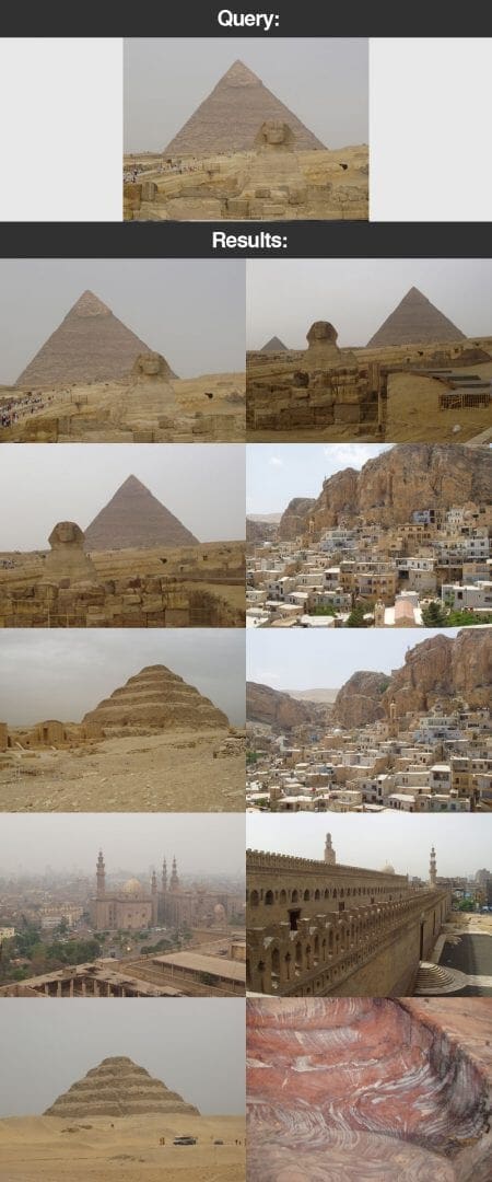
The first image you’ll see is our query image of the Egyptian pyramids. Our goal is to find similar images in our dataset. As you can see, we have clearly found the other photos of the dataset from when we visited the pyramids.
We also spent some time visiting other areas of Egypt. Let’s try another query image:
$ python search.py --index index.csv --query queries/115100.png --result-path dataset
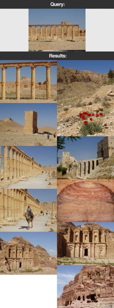
Be sure to pay close attention to our query image image. Notice how the sky is a brilliant shade of blue in the upper regions of the image. And notice how we have brown and tan desert and buildings at the bottom and center of the image.
And sure enough, in our results the images returned to us have blue sky in the upper regions and tan/brown desert and structures at the bottom.
The reason for this is because of our region-based color histogram descriptor that we detailed earlier in this post. By utilizing this image descriptor we have been able to perform a crude form of localization, providing our color histogram with hints as to “where” the pixel intensities occurred in the image.
Next up on our vacation we stopped at the beach. Execute the following command to search for beach photos:
$ python search.py --index index.csv --query queries/103300.png --result-path dataset
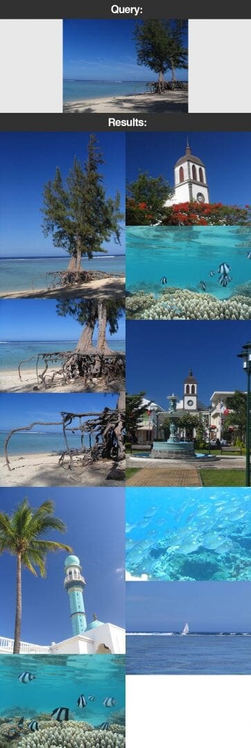
Notice how the first three results are from the exact same location on the trip to the beach. And the rest of the result images contain shades of blue.
Of course, no trip to the beach is complete without scubadiving:
$ python search.py --index index.csv --query queries/103100.png --result-path dataset
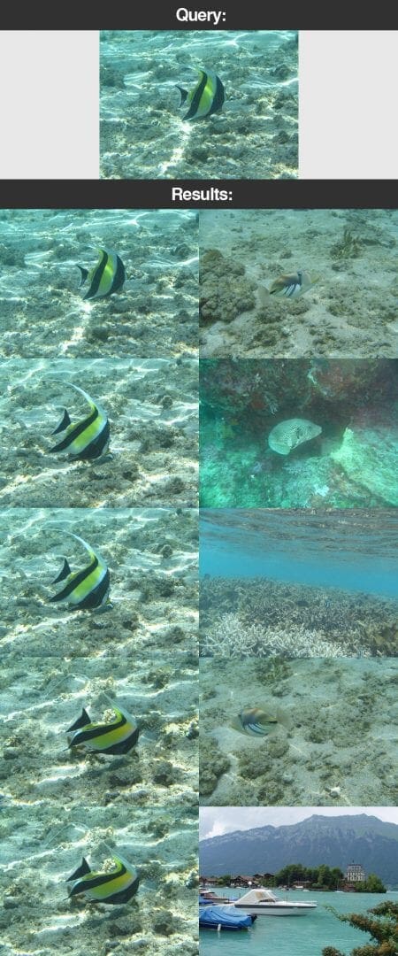
The results from this search are particularly impressive. The top 5 results are of the same fish — and all but one of the top 10 results are from the underwater excursion.
Finally, after a long day, it’s time to watch the sunset:
$ python search.py --index index.csv --query queries/127502.png --result-path dataset
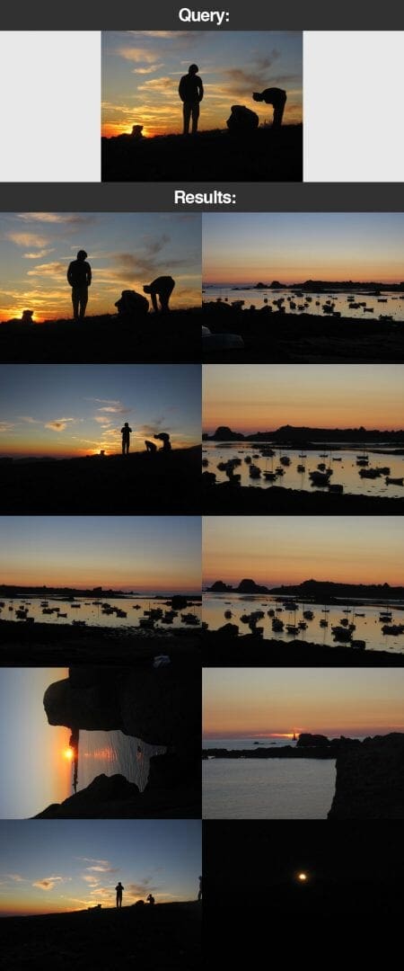
These search results are also quite good — all of the images returned are of the sunset at dusk.
So there you have it! Your first image search engine.
What's next? We recommend PyImageSearch University.
86+ total classes • 115+ hours hours of on-demand code walkthrough videos • Last updated: May 2026
★★★★★ 4.84 (128 Ratings) • 16,000+ Students Enrolled
I strongly believe that if you had the right teacher you could master computer vision and deep learning.
Do you think learning computer vision and deep learning has to be time-consuming, overwhelming, and complicated? Or has to involve complex mathematics and equations? Or requires a degree in computer science?
That’s not the case.
All you need to master computer vision and deep learning is for someone to explain things to you in simple, intuitive terms. And that’s exactly what I do. My mission is to change education and how complex Artificial Intelligence topics are taught.
If you're serious about learning computer vision, your next stop should be PyImageSearch University, the most comprehensive computer vision, deep learning, and OpenCV course online today. Here you’ll learn how to successfully and confidently apply computer vision to your work, research, and projects. Join me in computer vision mastery.
Inside PyImageSearch University you'll find:
- ✓ 86+ courses on essential computer vision, deep learning, and OpenCV topics
- ✓ 86 Certificates of Completion
- ✓ 115+ hours hours of on-demand video
- ✓ Brand new courses released regularly, ensuring you can keep up with state-of-the-art techniques
- ✓ Pre-configured Jupyter Notebooks in Google Colab
- ✓ Run all code examples in your web browser — works on Windows, macOS, and Linux (no dev environment configuration required!)
- ✓ Access to centralized code repos for all 540+ tutorials on PyImageSearch
- ✓ Easy one-click downloads for code, datasets, pre-trained models, etc.
- ✓ Access on mobile, laptop, desktop, etc.
Summary
In this blog post we explored how to build an image search engine to make our vacation photos search-able.
We utilized a color histogram to characterize the color distribution of our photos. Then, we indexed our dataset using our color descriptor, extracting color histograms from each of the images in the dataset.
To compare images we utilized the chi-squared distance, a popular choice when comparing discrete probability distributions.
From there, we implemented the necessary logic to accept a query image and then return relevant results.
Next Steps
So what are the next steps?
Well as you can see, the only way to interact with our image search engine is via the command line — that’s not very attractive.
In the next post we’ll explore how to wrap our image search engine in a Python web-framework to make it easier and sexier to use.

Download the Source Code and FREE 17-page Resource Guide
Enter your email address below to get a .zip of the code and a FREE 17-page Resource Guide on Computer Vision, OpenCV, and Deep Learning. Inside you'll find my hand-picked tutorials, books, courses, and libraries to help you master CV and DL!

