Update – January 27, 2015: Based on the feedback from commenters, I have updated the source code in the download to include the original MNIST dataset! No external downloads required!
Update – March 2015, 2015: The nolearn package has now deprecated and removed the dbn module. When you go to install the nolearn package, be sure to clone down the repository, checkout the 0.5b1 version, and then install it. Do not install the current version without first checking out the 0.5b1 version! In the future I will post an update on how to use the updated nolearn package!
Deep learning.
This probably isn’t the first time you’ve heard of it. It’s everywhere. In academic papers. On /r/machinelearning. On DataTau. On Hacker News. And even on primetime TV.
Now I’m not exactly a wagering man, but I bet that after my long-winded rant on getting off the deep learning bandwagon, the last thing you would expect me to do is write a post on Deep Learning, right?
Well. Let’s back up a step.
Remember, that post wasn’t saying that deep learning is bad or should be avoided — in fact, quite the contrary!
Instead, the post was simply a reminder that deep learning is still just a tool.
And with every tool, there is a time and a place to use it. Just because you have a “hammer”, doesn’t mean that every problem you come across will be a “nail”. It takes a conscientious effort to pick the right tool for the job.
Anyway, one of my favorite deep learning packages for Python is nolearn.
It’s beautiful. It’s simple. And if you’re familiar with scikit-learn, then you’ll feel right at home. The models included in nolearn have implemented the fit and predict functions just like scikit-learn, and the output predictions are even compatible with the scikit-learn metric functions.
Really cool, right?
Read on to find out how to utilize the nolearn package to construct a Deep Belief Network.
OpenCV and Python versions:
This example will run on Python 2.7 and OpenCV 2.4.X/OpenCV 3.0+.
Getting Started with Deep Learning and Python

So in this blog post we’ll review an example of using a Deep Belief Network to classify images from the MNIST dataset, a dataset consisting of handwritten digits. The MNIST dataset is extremely well studied and serves as a benchmark for new models to test themselves against.
However, in my opinion, this benchmark doesn’t necessarily translate into real-world viability. And this is mainly due to the dataset itself where each and every image has been pre-processed — including cropping, clean thresholding, and centering.
In the real-world, your dataset will not be as “nice” as the MNIST dataset. Your digits won’t be as cleanly pre-processed.
Still, this is a great starting point to get our feet wet utilizing Deep Belief Networks and nolearn .
Deep Learning Concepts and Assumptions
Deep learning is all about hierarchies and abstractions. These hierarchies are controlled by the number of layers in the network along with the number of nodes per layer. Adjusting the number of layers and nodes per layer can be used to provide varying levels of abstraction.
In general, the goal of deep learning is to take low level inputs (feature vectors) and then construct higher and higher level abstract “concepts” through the composition of layers. The assumption here is that the data follows some sort of underlying pattern generated by many interactions between different nodes on many different layers of the network.
Now that we have a high level understanding of Deep Learning concepts and assumptions, let’s look at some definitions to aide us in our learning.
The Input Layer, Hidden Layers, and Output Layer

Before we get to the code, let’s quickly discuss what Deep Belief Networks are, along with a bit of terminology.
This review is by no means meant to be complete and exhaustive. And in some cases I am greatly simplifying the details. But that’s okay. This is meant to be a gentle introduction to DBNs and not a hardcore review with tons of mathematical notation. If that’s what you’re looking for, then sorry, this isn’t the post for you. I would suggest reading up on the DeepLearning.net Tutorials (trust me, they are really good, but if this is your first exposure to deep learning, you might want to get through this post first).
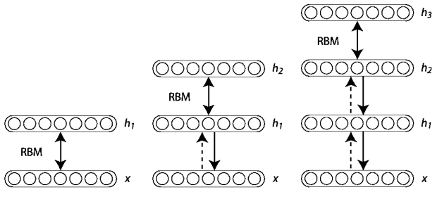
Deep Belief Networks consist of multiple layers, or more concretely, a hierarchy of unsupervised Restricted Boltzmann Machines (RBMs) where the output of each RBM is used as input to the next.
The major breakthrough came in 2006 when Hinton et al. published their A Fast Learning Algorithm for Deep Belief Networks paper. Their seminal work demonstrated that each of the hidden layers in a neural net can be treated as an unsupervised Restricted Boltzmann Machine with a supervised back-propagation step for fine-tuning. Furthermore, these RBMs can be trained greedily — and thus were feasible as highly scalable and efficient machine learning models.
This notion of efficiency was further demonstrated in the coming years where Deep Nets have been trained on GPUs rather than CPUs leading to a reduction of training time by over an order of magnitude. What once took weeks, now takes only days.
From there, deep learning has taken off.
But before we get too far, let’s quickly discuss this concept of “layers” in our DBN.
Input Layer
The first layer is our is a type of visible layer called an input layer. This layer contains an input node for each of the entries in our feature vector.
For example, in the MNIST dataset each image is 28 x 28 pixels. If we use the raw pixel intensities for the images, our feature vector would be of length 28 x 28 = 784, thus there would be 784 nodes in the input layer.
Hidden Layer
From there, these nodes connect to a series of hidden layers. In the most simple terms, each hidden layer is an unsupervised Restricted Boltzmann Machine where the output of each RBM in the hidden layer sequence is used as input to the next.
The final hidden layer then connects to an output layer.
Output Layer
Finally, we have our another visible layer called the output layer. This layer contains the output probabilities for each class label. For example, in our MNIST dataset we have 10 possible class labels (one for each of the digits 1-9). The output node that produces the largest probability is chosen as the overall classification.
Of course, we could always sort the output probabilities and choose all class labels that fall within some epsilon of the largest probability — doing this is a good way to find the most likely class labels rather than simply choosing the one with the largest probability. In fact, this is exactly what is done for many of the popular deep learning challenges, including ImageNet.
Now that we have some terminology, we can jump into the code.
Utilizing a Deep Belief Network in Python
Alright, time for the fun part — let’s write some code.
It is important to note that this tutorial (by in large) is based on the excellent example on the nolearn website. My goal here is to simply take the example, tweak it slightly, as well as throw in a few extra demonstrations — and provide a detailed review of the code, of course.
Anyway, open up a new file, name it dbn.py , and let’s get started.
# import the necessary packages
from sklearn.cross_validation import train_test_split
from sklearn.metrics import classification_report
from sklearn import datasets
from nolearn.dbn import DBN
import numpy as np
import cv2
We’ll start by importing the packages that we’ll need. We’ll import train_test_split (to generate our training and testing splits of the MNIST dataset) and classification_report (to display a nicely formatted table of accuracies) from the scikit-learn package. We’ll import the dataset module from scikit-learn to download the MNIST dataset.
Next up, we’ll import our Deep Belief Network implementation from the nolearn package.
And finally we’ll wrap up our import statements by importing NumPy for numerical processing and cv2 for our OpenCV bindings.
Let’s go ahead and download the MNIST dataset:
# grab the MNIST dataset (if this is the first time you are running
# this script, this make take a minute -- the 55mb MNIST digit dataset
# will be downloaded)
print "[X] downloading data..."
dataset = datasets.fetch_openml("mnist_784", version=1)
We make a call to the fetch_mldata function on Line 13 that downloads the original MNIST dataset from the mldata.org repository.
The actual dataset is roughly 55mb so it may take a few seconds to download. However, once the dataset is downloaded it is cached locally on your machine so you will not have to download it again.
If you take the time to examine the data, you’ll notice that each feature vector contains 784 entries in the range [0, 255]. These values are the grayscale pixel intensities of the flattened 28 x 28 image. Background pixels are black (0) whereas foreground pixels appear to be lighter shades of gray or white.
Time to generate our training and testing splits:
# scale the data to the range [0, 1] and then construct the training
# and testing splits
(trainX, testX, trainY, testY) = train_test_split(
	dataset.data / 255.0, dataset.target.astype("int0"), test_size = 0.33)
In order to train our Deep Belief network, we’ll need two sets of data — a set for training our algorithm and a set for evaluating or testing the performance of the classifier.
We perform the split on Lines 17 and 18 by making call to train_test_split. The first argument we specify is the data itself, which we scale to be in range [0, 1.0]. The Deep Belief Network assumes that our data is scaled in the range [0, 1.0] so this is a necessary step.
We then specify the “target” or the “class labels” for each feature vector as the second argument.
The last argument to train_test_split is the size of our testing set. We’ll utilize 33% of the data for testing, while the remaining 67% will be utilized for training our Deep Belief Network.
Speaking of training the Deep Belief Network, let’s go ahead and do that:
# train the Deep Belief Network with 784 input units (the flattened,
# 28x28 grayscale image), 300 hidden units, 10 output units (one for
# each possible output classification, which are the digits 1-10)
dbn = DBN(
	[trainX.shape[1], 300, 10],
	learn_rates = 0.3,
	learn_rate_decays = 0.9,
	epochs = 10,
	verbose = 1)
dbn.fit(trainX, trainY)
We initialize our Deep Belief Network on Lines 23-28.
The first argument details the structure of our network, represented as a list. The first entry in the list is the number of nodes in our input layer. We’ll want to have an input node for each entry in our feature vector list, so we’ll specify the length of the feature vector for this value.
Our input layer will now feed forward into our second entry in the list, a hidden layer. This hidden layer will be represented as RBM with 300 nodes.
Finally, the output of the 300 node hidden layer will be fed into the output layer, which consists of an output for each of the class labels.
We can then define our learn_rate , which is the learning rate of the algorithm, the decay of the learn rate (learn_rate_decays ), the number of epochs , or iterations of the training data, and the verbosity level.
Both learn_rates and learn_rates_decays can be specified as a single floating point values or a list of floating point values. If you specify only a single value, this learning rate/decay rate will be applied to all layers in the network. If you specify a list of values, the the corresponding learning rate and decay rate will be used for the respective layers.
Training the actual algorithm takes place on Line 29. If you have a slow machine, you way want to make a cup of coffee or go for a quick walk during this time.
Now that our Deep Belief Network is trained, let’s go ahead and evaluate it:
# compute the predictions for the test data and show a classification
# report
preds = dbn.predict(testX)
print classification_report(testY, preds)
Here we make a call to the predict method of the network on Line 33 which takes our testing data and makes predictions regarding which digit each image contains. If you have worked with scikit-learn at all, then this should feel very natural and comfortable.
We then present a table of accuracies on Line 34.
Finally, I thought it might be interesting to inspect images individually rather than on aggregate as a further demonstration of the network:
# randomly select a few of the test instances
for i in np.random.choice(np.arange(0, len(testY)), size = (10,)):
	# classify the digit
	pred = dbn.predict(np.atleast_2d(testX[i]))

	# reshape the feature vector to be a 28x28 pixel image, then change
	# the data type to be an unsigned 8-bit integer
	image = (testX[i] * 255).reshape((28, 28)).astype("uint8")

	# show the image and prediction
	print "Actual digit is {0}, predicted {1}".format(testY[i], pred[0])
	cv2.imshow("Digit", image)
	cv2.waitKey(0)
On Line 37 we loop over 10 randomly chosen feature vectors from the test data.
We then predict the digit in the image on Line 39.
To display our image on screen, we need to reshape it on Line 43. Since our data is in the range [0, 1.0], we first multiply by 255 to put it back in the range [0, 255], change the shape to be a 28 x 28 pixel image, and then change the data type from floating point to an unsigned 8-bit integer.
Finally, we display the results of the prediction on Lines 46-48.
Results
Now that the code is done, let’s look at the results.
Fire up a shell, navigate to your dbn.py file, and issue the following command:
$ python dbn.py
gnumpy: failed to import cudamat. Using npmat instead. No GPU will be used.
[X] downloading data...
[DBN] fitting X.shape=(46900, 784)
[DBN] layers [784, 300, 10]
[DBN] Fine-tune...
100%
Epoch 1:
  loss 0.288535176023
  err  0.0842298497268
  (0:00:04)
100%
Epoch 2:
  loss 0.170946833078
  err  0.0495645491803
  (0:00:05)
100%
Epoch 3:
  loss 0.127217275595
  err  0.0362662226776
  (0:00:04)
100%
Epoch 4:
  loss 0.0930059491925
  err  0.0268954918033
  (0:00:05)
100%
Epoch 5:
  loss 0.0732877224143
  err  0.0234161543716
  (0:00:04)
100%
Epoch 6:
  loss 0.0563644782051
  err  0.0173539959016
  (0:00:04)
100%
Epoch 7:
  loss 0.0383996891073
  err  0.012487192623
  (0:00:05)
100%
Epoch 8:
  loss 0.027456679965
  err  0.00817537568306
  (0:00:05)
100%
Epoch 9:
  loss 0.0208912373799
  err  0.00589139344262
  (0:00:05)
100%
Epoch 10:
  loss 0.0203280455254
  err  0.00616888661202
  (0:00:05)
             precision    recall  f1-score   support

          0       0.98      0.99      0.99      2280
          1       0.99      0.98      0.99      2617
          2       0.98      0.98      0.98      2285
          3       0.97      0.98      0.97      2356
          4       0.98      0.98      0.98      2268
          5       0.98      0.97      0.98      2133
          6       0.98      0.98      0.98      2217
          7       0.99      0.98      0.98      2430
          8       0.97      0.97      0.97      2255
          9       0.97      0.97      0.97      2259

avg / total       0.98      0.98      0.98     23100
Here you can see that our Deep Belief Network is trained over 10 epochs (iterations over the training data). At each iteration our our loss function is minimized and the error on the training set is lower.
Taking a look at our classification report we see that we have obtained 98% accuracy (the precision column) on our testing set. As you can see, the “1” and “7” digits was accurately classified 99% of the time. We could have perhaps obtained higher accuracy for the other digits had we let our network train for more epochs.
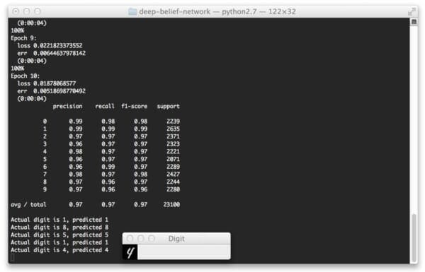
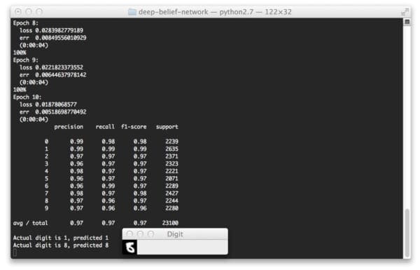
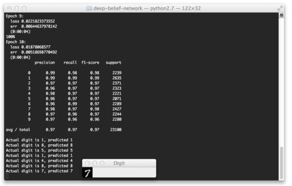
And below we can see some screenshots of our Deep Belief Network correctly classifying the digit in their respective images.
Note: You’ll notice that the loss, error, and accuracy values do not 100% match the output above. That is because I gathered these sample images on a separate run of the algorithm. Deep Belief Networks are stochastic algorithms, meaning that the algorithm utilizes random variables; thus, it is normal to obtain slightly different results when running the learning algorithm multiple times. To account for this, it is normal to obtain multiple sets of results and average them together prior to reporting final accuracies.

Here we can see that we have correctly classified the “1” digit.

Again, we can see that our digit is correctly classified.
But take a look at this “8” digit below. This is far from a “legible digit”, but the Deep Belief Network is still able to sort it out:

Finally, let’s try a “7”:

Yep, that one is correctly classified as well!
What's next? We recommend PyImageSearch University.
86+ total classes • 115+ hours hours of on-demand code walkthrough videos • Last updated: May 2026
★★★★★ 4.84 (128 Ratings) • 16,000+ Students Enrolled
I strongly believe that if you had the right teacher you could master computer vision and deep learning.
Do you think learning computer vision and deep learning has to be time-consuming, overwhelming, and complicated? Or has to involve complex mathematics and equations? Or requires a degree in computer science?
That’s not the case.
All you need to master computer vision and deep learning is for someone to explain things to you in simple, intuitive terms. And that’s exactly what I do. My mission is to change education and how complex Artificial Intelligence topics are taught.
If you're serious about learning computer vision, your next stop should be PyImageSearch University, the most comprehensive computer vision, deep learning, and OpenCV course online today. Here you’ll learn how to successfully and confidently apply computer vision to your work, research, and projects. Join me in computer vision mastery.
Inside PyImageSearch University you'll find:
- ✓ 86+ courses on essential computer vision, deep learning, and OpenCV topics
- ✓ 86 Certificates of Completion
- ✓ 115+ hours hours of on-demand video
- ✓ Brand new courses released regularly, ensuring you can keep up with state-of-the-art techniques
- ✓ Pre-configured Jupyter Notebooks in Google Colab
- ✓ Run all code examples in your web browser — works on Windows, macOS, and Linux (no dev environment configuration required!)
- ✓ Access to centralized code repos for all 540+ tutorials on PyImageSearch
- ✓ Easy one-click downloads for code, datasets, pre-trained models, etc.
- ✓ Access on mobile, laptop, desktop, etc.
Summary
So there you have it — an brief, gentle introduction to Deep Belief Networks.
In this post we reviewed the structure of a Deep Belief Network (at a very high level) and looked at the nolearn Python package.
We then utilized nolearn to train and evaluate a Deep Belief Network on the MNIST dataset.
If this is your first experience with DBNs, I highly recommend that you spend the next few days researching and reading up on Artificial Neural Networks (ANNs); specifically, feed-forward networks, the back-propagation algorithm, and Restricted Boltzmann Machines.
Honestly, if you are serious about exploring Deep Learning, the algorithms I mentioned above are required, non-optional reading!
You won’t get very far into deep learning without reading up on these techniques. And don’t be afraid of the academic papers either! That’s where you’ll find all the gory details.
What’s Next?
Training a Deep Belief Network on a CPU can take a long, long time.
Luckily, we can speed up the training process using our GPUs, leading to training times being reduced by an order of magnitude or more.
In my next post I’ll show you how to setup your system to train a Deep Belief Network on your GPU. I think the speedup in training time will be quite surprising…
Be sure to enter your email address in the form at the bottom of this post to be updated when the next post goes live! You definitely won’t want to miss it.
Interested in Handwriting Recognition?

Did you enjoy this post on handwriting recognition?
If so, you’ll definitely want to check out my Practical Python and OpenCV book!
Chapter 6, Handwriting Recognition with HOG details the techniques the pro’s use…allowing you to become a pro yourself! From pre-processing the digit images, utilizing the Histogram of Oriented Gradients (HOG) image descriptor, and training a Linear SVM, this chapter covers handwriting recognition from front-to-back.
Simply put — if you loved this blog post, you’ll love this book.
Sound interesting?
Click here to pickup a copy of the Practical Python and OpenCV

Download the Source Code and FREE 17-page Resource Guide
Enter your email address below to get a .zip of the code and a FREE 17-page Resource Guide on Computer Vision, OpenCV, and Deep Learning. Inside you'll find my hand-picked tutorials, books, courses, and libraries to help you master CV and DL!

