Are you ready to start building your first image search engine? Not so fast! Let’s first go over some basic image processing and manipulations that will come in handy along your image search engine journey. If you are already an image processing guru, this post will seem pretty boring to you, but give it a read none-the-less — you might pick up a trick or two.
OpenCV and Python versions:
This example will run on Python 2.7 and OpenCV 2.4.X/OpenCV 3.0+.
For this introduction to basic image processing, I’m going to assume that you have basic knowledge of how to create and execute Python scripts. I’m also going to assume that you have OpenCV installed. If you need help installing OpenCV, check out the quick start guides on the OpenCV website.
Continuing my obsession with Jurassic Park let’s use the Jurassic Park tour jeep as our example image to play with:

Go ahead and download this image to your computer. You’ll need it to start playing with some of the Python and OpenCV sample code.
Ready? Here we go.
First, let’s load the image and display it on screen:
# import the necessary packages
import cv2

# load the image and show it
image = cv2.imread("jurassic-park-tour-jeep.jpg")
cv2.imshow("original", image)
cv2.waitKey(0)
Executing this Python snippet gives me the following result on my computer:

As you can see, the image is now displaying. Let’s go ahead and break down the code:
- Line 2: The first line is just telling the Python interpreter to import the OpenCV package.
- Line 5: We are now loading the image off of disk. The
imreadfunctions returns a NumPy array, representing the image itself. - Line 6 and 7: A call to
imshowdisplays the image on our screen. The first parameter is a string, the “name” of our window. The second parameter is a reference to the image we loaded off disk on Line 5. Finally, a call towaitKeypauses the execution of the script until we press a key on our keyboard. Using a parameter of “0” indicates that any keypress will un-pause the execution.
Just loading and displaying an image isn’t very interesting. Let’s resize this image and make it much smaller. We can examine the dimensions of the image by using the shape attribute of the image, since the image is a NumPy array after-all:
# print the dimensions of the image
print image.shape
When executing this code, we see that (388, 647, 3) is outputted to our terminal. This means that the image has 388 rows, 647 columns, and 3 channels (the RGB components). When we write matrices, it is common to write them in the form (# of rows x # of columns) — which is the same way you specify the matrix size in NumPy.
However, when working with images this can become a bit confusing since we normally specify images in terms of width x height. Looking at the shape of the matrix, we may think that our image is 388 pixels wide and 647 pixels tall. However, this would be incorrect. Our image is actually 647 pixels wide and 388 pixels tall, implying that the height is the first entry in the shape and the width is the second. This little may be a bit confusing if you’re just getting started with OpenCV and is important to keep in mind.
Since we know that our image is 647 pixels wide, let’s resize it and make it 100 pixels wide:
# we need to keep in mind aspect ratio so the image does
# not look skewed or distorted -- therefore, we calculate
# the ratio of the new image to the old image
r = 100.0 / image.shape[1]
dim = (100, int(image.shape[0] * r))

# perform the actual resizing of the image and show it
resized = cv2.resize(image, dim, interpolation = cv2.INTER_AREA)
cv2.imshow("resized", resized)
cv2.waitKey(0)
Executing this code we can now see that the new resized image is only 100 pixels wide:

Let’s breakdown the code and examine it:
- Line 15 and 16: We have to keep the aspect ratio of the image in mind, which is the proportional relationship of the width and the height of the image. In this case, we are resizing the image to have a 100 pixel width, therefore, we need to calculate
r, the ratio of the new width to the old width. Then, we construct the new dimensions of the image by using 100 pixels for the width, and r x the old image height. Doing this allows us to maintain the aspect ratio of the image. - Lines 19-21: The actual resizing of the image happens here. The first parameter is the original image that we want to resize and the second argument is the our calculated dimensions of the new image. The third parameter tells us the algorithm to use when resizing. Don’t worry about that for now. Finally, we show the image and wait for a key to be pressed.
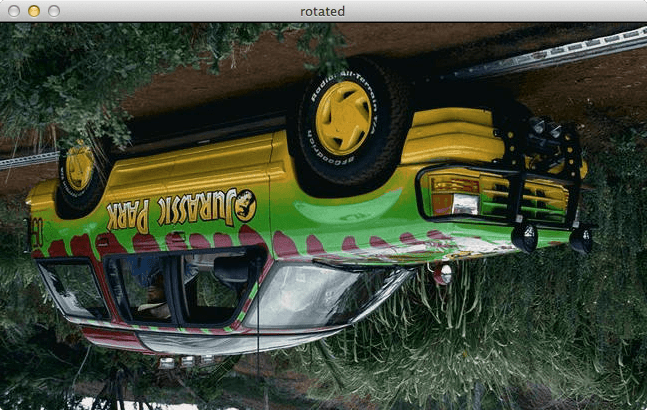
Resizing an image wasn’t so bad. Now, let’s pretend that we are the Tyrannosaurus Rex from the Jurassic Park movie — let’s flip this jeep upside down:
# grab the dimensions of the image and calculate the center
# of the image
(h, w) = image.shape[:2]
center = (w / 2, h / 2)

# rotate the image by 180 degrees
M = cv2.getRotationMatrix2D(center, 180, 1.0)
rotated = cv2.warpAffine(image, M, (w, h))
cv2.imshow("rotated", rotated)
cv2.waitKey(0)
So what does the jeep look like now? You guessed it — flipped upside down.

This is the most involved example that we’ve looked at thus far. Let’s break it down:
- Line 25: For convenience, we grab the width and height of the image and store them in their respective variables.
- Line 26: Calculate the center of the image — we simply divide the width and height by 2.
- Line 29: Compute a matrix that can be used for rotating (and scaling) the image. The first argument is the center of the image that we computed. If you wanted to rotate the image around any arbitrary point, this is where you would supply that point. The second argument is our rotation angle (in degrees). And the third argument is our scaling factor — in this case, 1.0, because we want to maintain the original scale of the image. If we wanted to halve the size of the image, we would use 0.5. Similarly, if we wanted to double the size of the image, we would use 2.0.
- Line 30: Perform the actual rotation, by suppling the image, the rotation matrix, and the output dimensions.
- Lines 31-32: Show the rotated image.
Rotating an image is definitely the most complicated image processing technique we’ve done thus far.
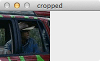
Let’s move on to cropping the image and grab a close-up of Grant:
# crop the image using array slices -- it's a NumPy array
# after all!
cropped = image[70:170, 440:540]
cv2.imshow("cropped", cropped)
cv2.waitKey(0)
Take a look at Grant. Does he look like he sees a sick Triceratops?

Cropping is dead as Dennis Nedry in Python and OpenCV. All we are doing is slicing arrays. We first supply the startY and endY coordinates, followed by the startX and endX coordinates to the slice. That’s it. We’ve cropped the image!
As a final example, let’s save the cropped image to disk, only in PNG format (the original was a JPG):
# write the cropped image to disk in PNG format
cv2.imwrite("thumbnail.png", cropped)
All we are doing here is providing the path to the file (the first argument) and then the image we want to save (the second argument). It’s that simple.

As you can see, OpenCV takes care of changing formats for us.
And there you have it! Basic image manipulations in Python and OpenCV! Go ahead and play around with the code yourself and try it out on your favorite Jurassic Park images.
What's next? We recommend PyImageSearch University.
86 total classes • 115+ hours of on-demand code walkthrough videos • Last updated: October 2024
★★★★★ 4.84 (128 Ratings) • 16,000+ Students Enrolled
I strongly believe that if you had the right teacher you could master computer vision and deep learning.
Do you think learning computer vision and deep learning has to be time-consuming, overwhelming, and complicated? Or has to involve complex mathematics and equations? Or requires a degree in computer science?
That’s not the case.
All you need to master computer vision and deep learning is for someone to explain things to you in simple, intuitive terms. And that’s exactly what I do. My mission is to change education and how complex Artificial Intelligence topics are taught.
If you're serious about learning computer vision, your next stop should be PyImageSearch University, the most comprehensive computer vision, deep learning, and OpenCV course online today. Here you’ll learn how to successfully and confidently apply computer vision to your work, research, and projects. Join me in computer vision mastery.
Inside PyImageSearch University you'll find:
- ✓ 86 courses on essential computer vision, deep learning, and OpenCV topics
- ✓ 86 Certificates of Completion
- ✓ 115+ hours of on-demand video
- ✓ Brand new courses released regularly, ensuring you can keep up with state-of-the-art techniques
- ✓ Pre-configured Jupyter Notebooks in Google Colab
- ✓ Run all code examples in your web browser — works on Windows, macOS, and Linux (no dev environment configuration required!)
- ✓ Access to centralized code repos for all 540+ tutorials on PyImageSearch
- ✓ Easy one-click downloads for code, datasets, pre-trained models, etc.
- ✓ Access on mobile, laptop, desktop, etc.

Download the Source Code and FREE 17-page Resource Guide
Enter your email address below to get a .zip of the code and a FREE 17-page Resource Guide on Computer Vision, OpenCV, and Deep Learning. Inside you'll find my hand-picked tutorials, books, courses, and libraries to help you master CV and DL!


