Train YOLO26 on a Custom Dataset with YOLOE-26 Auto-Labeling

---

Train YOLO26 on a Custom Dataset with YOLOE-26 Auto-Labeling

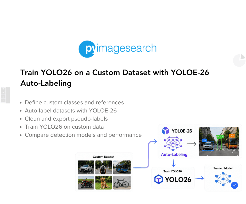
In this lesson, you will learn how to use YOLOE-26 visual prompting to auto-label a custom dataset, clean pseudo-labels, export YOLO training data, and fine-tune YOLO26 for class-specific object detection.

This lesson is the last in a 2-part series on YOLOE-26 and open-vocabulary detection:

1. YOLO26 Open-Vocabulary Object Detection with YOLOE-26
2. Train YOLO26 on a Custom Dataset with YOLOE-26 Auto-Labeling (this tutorial)

To learn how to bootstrap a custom detector with YOLOE-26 and fine-tune YOLO26 on your own classes, just keep reading.

---

In the first lesson, we stayed in the open-vocabulary world. We learned what YOLOE (Wang et al., 2025) introduced, how YOLOE-26 extends those ideas into the YOLO26 family, and how text prompts, visual prompts, and prompt-free inference change the way we talk to a detector.

This lesson answers the next practical question:

What do we do once YOLOE-26 can already find the object we care about?

One good answer is to use it as a bootstrap engine.

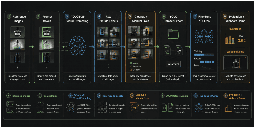
Instead of labeling a small custom dataset box by box from scratch, we can use YOLOE-26 visual prompting to generate pseudo-labels, clean the noisy ones, export the results in standard YOLO format, and then fine-tune a smaller closed-set YOLO26 detector for the final deployment step.

That is exactly what we will do here.

We are going to build a small 2-class detector for 2 perfume bottles:

• creed_aventus
• dior_elixir

In this lesson, we will learn:

• how to structure a small pseudo-labeling workflow around YOLOE-26 visual prompts
• how to define custom classes and reference images in a reusable config
• how to generate raw pseudo-labels and consolidate duplicate detections
• how to clean noisy labels and manually fix the small number of images that still fail
• how to export the cleaned labels into standard YOLO training format
• how to fine-tune yolo26s.pt on the resulting dataset
• how to compare baseline YOLO26, YOLOE-26, and the fine-tuned detector honestly

---

Auto-Labeling a Custom Dataset for YOLO26 Object Detection

In Lesson 1, we showed that YOLOE-26 can find objects from prompts. That is already useful on its own.

But many real projects eventually want something narrower and more product-like:

• a fixed label list
• a small deployment artifact
• no prompt setup at inference time
• a detector that can keep improving as we correct more data

That is where a closed-set fine-tuned detector still makes sense.

In this lesson, the target problem is intentionally small and concrete. We want to detect 2 visually distinct bottles from our own photos, not from a public dataset. No Common Objects in Context (COCO) class will solve that directly. A standard YOLO26 model can usually tell us that the image contains a bottle-like object, but it cannot natively distinguish which bottle it is.

YOLOE-26 gives us a way to bridge that gap. We can show it clean reference examples of each bottle, let it search the rest of our images for similar objects, and then turn those predictions into a first-pass training set.

The important point is that we are not pretending the pseudo-labels will be perfect. They almost never are. We are using them to replace most of the manual labeling work, not all of it.

---

Would you like immediate access to 3,457 images curated and labeled with hand gestures to train, explore, and experiment with … for free? Head over to Roboflow and get a free account to grab these hand gesture images.

---

Configuring Your Development Environment

To follow this guide, we need a Python environment with Ultralytics, OpenCV, Pillow, NumPy, and PyYAML installed.

$ pip install -U ultralytics opencv-python pillow numpy pyyaml

If you need help configuring your development environment for OpenCV, we highly recommend reading our pip install OpenCV guide. It will have you up and running in minutes.

---

Need Help Configuring Your Development Environment?

All that said, are you:

• Short on time?
• Learning on your employer’s administratively locked system?
• Wanting to skip the hassle of fighting with the command line, package managers, and virtual environments?
• Ready to run the code immediately on your Windows, macOS, or Linux system?

Then join PyImageSearch University today!

Gain access to Jupyter Notebooks for this tutorial and other PyImageSearch guides pre-configured to run on Google Colab’s ecosystem right in your web browser! No installation required.

And best of all, these Jupyter Notebooks will run on Windows, macOS, and Linux!

---

Project Structure

We first need to review our project directory structure.

Start by accessing this tutorial’s “Downloads” section to retrieve the source code and example images.

From there, take a look at the directory structure:

yoloe26-bootstrap-finetuning/
├── configs/
│   ├── classes.yaml
│   └── reference_prompts.json
├── data/
│   ├── raw/
│   │   ├── reference/
│   │   │   ├── bottle_a/
│   │   │   └── bottle_b/
│   │   ├── train/
│   │   └── val/
│   ├── interim/
│   │   ├── pseudo_labels/
│   │   ├── cleaned_labels/
│   │   └── review_exports/
│   └── processed/
│       └── yolo_dataset/
│           ├── data.yaml
│           ├── images/
│           │   ├── train/
│           │   └── val/
│           └── labels/
│               ├── train/
│               └── val/
├── outputs/
│   ├── checkpoints/
│   │   └── yolo26s_perfume_pilot/
│   ├── figures/
│   │   └── comparison_val/
│   ├── metrics/
│   └── previews/
├── scripts/
│   ├── 01_build_reference_prompts.py
│   ├── 02_run_pseudo_labeling.py
│   ├── 03_clean_pseudo_labels.py
│   ├── 04_export_yolo_dataset.py
│   ├── 05_manual_fix_cleaned_labels.py
│   ├── 05_train_yolo26.py
│   ├── 06_webcam_demo.py
│   └── 07_evaluate_models.py
├── src/
│   └── config.py
└── yolo26s.pt

Before we run anything, let us anchor the workflow to the files that matter most:

• configs/classes.yaml: defines the classes, reference-image filenames, and the default pseudo-label confidence threshold.
• src/config.py: centralizes path handling, class loading, and split discovery.
• scripts/01_build_reference_prompts.py: lets us draw 1 or more prompt boxes on the reference images.
• scripts/02_run_pseudo_labeling.py: runs YOLOE-26 visual prompting over a split and saves raw overlays.
• scripts/03_clean_pseudo_labels.py: applies confidence filtering and overlap suppression.
• scripts/05_manual_fix_cleaned_labels.py: lets us patch the small number of images that still need human correction.
• scripts/04_export_yolo_dataset.py: converts the cleaned detections into YOLO .txt label files and data.yaml.
• scripts/05_train_yolo26.py: fine-tunes a closed-set YOLO26 detector.
• scripts/06_webcam_demo.py: loads the fine-tuned checkpoint for a live qualitative sanity check.
• scripts/07_evaluate_models.py: generates side-by-side comparisons of baseline YOLO26, YOLOE-26, and the fine-tuned model.

That file split is worth noticing. Instead of hiding the whole lesson inside a single notebook cell stream, we broke the workflow into small, repeatable stages. That makes the pipeline easier to rerun and easier to explain.

---

Step 1: Define Custom Object Classes and Reference Images

We start in configs/classes.yaml.

This file defines our 2 custom classes, the prompt reference images for each class, and the default pseudo-label confidence threshold:

project:
  model_path: "../yoloe-26s-seg.pt"
  default_split: "train"
  pseudo_label_confidence: 0.35

classes:
  - id: 0
    name: "creed_aventus"
    display_name: "Creed Aventus"
    reference_subdir: "bottle_a"
    reference_images:
      - "IMG_3825_Best.jpg"
      - "IMG_3826.jpg"
      - "IMG_3827.jpg"
      - "IMG_3849.JPG"

  - id: 1
    name: "dior_elixir"
    display_name: "Dior Sauvage Elixir"
    reference_subdir: "bottle_b"
    reference_images:
      - "IMG_3822_Best.jpg"
      - "IMG_3823.jpg"
      - "IMG_3824.jpg"
      - "IMG_3844.JPG"
      - "IMG_3846.JPG"
      - "IMG_3847.JPG"
      - "IMG_3848.JPG"

There are 2 practical design choices here.

First, we do not rely on a single reference image per class. We let each class carry a small bundle of references. That makes the visual prompting stage more robust when a bottle is seen from a different angle, at a different size, or under slightly different lighting.

Second, the label names are the names we want in the final detector. The filenames of the training images do not become labels. Only the class entries in this config and the exported YOLO annotations determine the training target.

src/config.py is the small plumbing layer that makes this ergonomic:

def load_classes(paths: ProjectPaths | None = None) -> list[ClassSpec]:
    paths = paths or get_paths()
    raw = load_yaml(paths.classes_yaml)
    class_specs: list[ClassSpec] = []
    for item in raw["classes"]:
        reference_images = item.get("reference_images")
        if reference_images is None:
            reference_images = [item["reference_image"]]
        class_specs.append(
            ClassSpec(
                id=int(item["id"]),
                name=str(item["name"]),
                display_name=str(item["display_name"]),
                reference_subdir=str(item["reference_subdir"]),
                reference_images=tuple(str(image_name) for image_name in reference_images),
                review_color_bgr=tuple(item["review_color_bgr"]),
            )
        )
    return class_specs

That helper is small, but it matters. Every later script reuses the same class definitions, paths, and split logic, so the whole pipeline stays consistent.

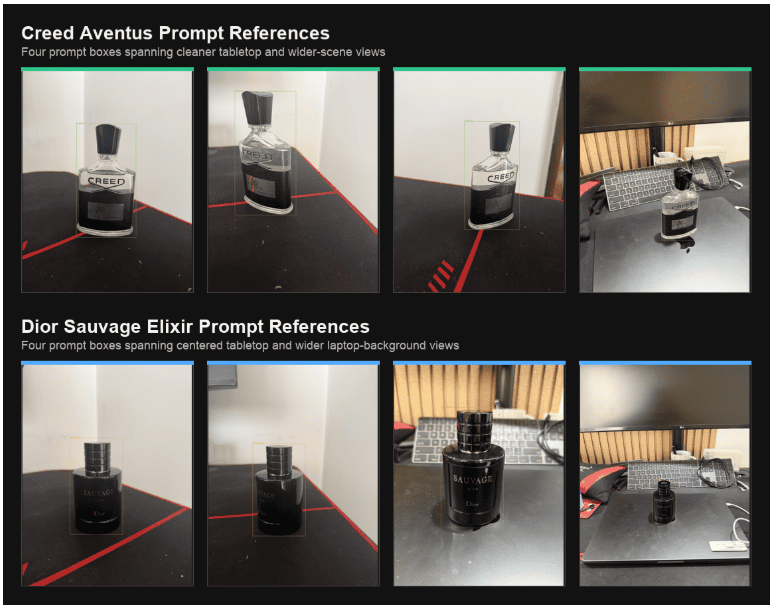
Note: The prompt boxes are intentionally thin in a few panels. Zoom in for a clearer view of the bounding boxes.

---

Step 2: Draw Visual Prompt Boxes for YOLOE-26 Auto-Labeling

Once the reference images exist, scripts/01_build_reference_prompts.py opens a region of interest (ROI) selector so we can draw 1 tight prompt box per reference image.

The core function is straightforward:

def select_prompt_box(image_path: Path, class_spec: ClassSpec, prompt_index: int, total_prompts: int) -> list[int]:
    image = cv2.imread(str(image_path))
    window_name = f"{class_spec.display_name} ({prompt_index}/{total_prompts})"
    roi = cv2.selectROI(window_name, image, showCrosshair=True, fromCenter=False)
    cv2.destroyAllWindows()
    x, y, w, h = roi
    return [int(x), int(y), int(x + w), int(y + h)]

This is one place where a graphical user interface (GUI) tool is exactly the right choice. We only do this once per reference image, and the output becomes a reusable JavaScript Object Notation (JSON) file (configs/reference_prompts.json) for every later step.

Run it like this:

python3 scripts/01_build_reference_prompts.py --overwrite

The script also saves preview overlays so we can visually confirm that the prompt boxes are tight and centered on the full bottle.

What reference_prompts.json Actually Stores

It is worth pausing here, because configs/reference_prompts.json becomes the contract between the interactive prompt-selection step and the automated pseudo-labeling step.

A simplified entry looks like this:

{
  "classes": {
    "creed_aventus": {
      "class_id": 0,
      "display_name": "Creed Aventus",
      "references": [
        {
          "reference_image": "data/raw/reference/bottle_a/IMG_3825_Best.jpg",
          "xyxy": [1365, 1432, 2874, 4306],
          "preview_image": "data/interim/review_exports/reference_prompts/creed_aventus_reference_prompt_01.jpg"
        }
      ]
    }
  }
}

The following 3 fields matter most:

• reference_image: tells later scripts which source image to use as the prompt image
• xyxy: stores the tight visual prompt box in pixel coordinates
• preview_image: gives us a saved sanity-check overlay we can inspect before running the full pipeline

This is a place where the codebase structure helps. We never have to redraw those boxes unless we deliberately want to change the prompt setup.

---

Step 3: Auto-Label a Custom Dataset with YOLOE-26 Visual Prompting

Now we can let YOLOE-26 do the first pass of the labeling work.

The heart of scripts/02_run_pseudo_labeling.py is the visual-prompt inference call:

model.set_classes([class_spec.name])
visual_prompts = {
    "bboxes": np.array([[x1, y1, x2, y2]], dtype=np.float32),
    "cls": np.array([0], dtype=np.int32),
}

results = model.predict(
    source=image_sources,
    refer_image=str(reference_image),
    visual_prompts=visual_prompts,
    predictor=YOLOEVPSegPredictor,
    conf=confidence,
    verbose=False,
)

This is the critical shift from Lesson 1 to Lesson 2.

In Lesson 1, visual prompting was an inference trick. Here, it becomes a dataset-building primitive.

We take each class, loop over its reference images, and run that visual prompt across the whole split. Every detection is saved with:

• image_rel_path
• class_id
• class_name
• confidence
• x1, y1, x2, y2

Because we are using multiple references per class, we also need a consolidation step. Otherwise, nearly identical prompt boxes can produce duplicate detections on the same image.

That is why the script includes consolidate_image_detections():

def consolidate_image_detections(
    detections: list[dict[str, object]],
    same_class_iou_threshold: float = 0.60,
    cross_class_iou_threshold: float = 0.80,
) -> list[dict[str, object]]:
    by_class: dict[str, list[dict[str, object]]] = defaultdict(list)
    for detection in detections:
        by_class[str(detection["class_name"])].append(detection)

    same_class_merged: list[dict[str, object]] = []
    for class_name in sorted(by_class):
        same_class_merged.extend(
            suppress_overlaps(by_class[class_name], iou_threshold=same_class_iou_threshold)
        )

    cross_class_merged = suppress_overlaps(
        same_class_merged,
        iou_threshold=cross_class_iou_threshold,
    )
    return sorted(cross_class_merged, key=lambda item: (int(item["class_id"]), -float(item["confidence"])))

That function ended up being more important than it may look at first glance. Once we started using several reference images per class, raw detections could accumulate quickly. The intersection over union (IoU)-based consolidation keeps only the strongest overlapping box and makes the review artifacts much easier to inspect.

Run the pseudo-labeling pass like this:

python3 scripts/02_run_pseudo_labeling.py --split train
python3 scripts/02_run_pseudo_labeling.py --split val

The script saves machine-readable JavaScript Object Notation (JSON) and comma-separated values (CSV) outputs, along with human-review artifacts:

• data/interim/pseudo_labels/<split>_raw_predictions.json
• data/interim/pseudo_labels/<split>_raw_predictions.csv
• data/interim/review_exports/raw_predictions/*.jpg

What One Raw Pseudo-Label Record Looks Like

The JSON output is designed to be both reviewable and script-friendly. A single image entry looks like this:

{
  "image_rel_path": "data/raw/train/session_02_bottle_b_solo/IMG_3859.JPG",
  "preview_image": "data/interim/review_exports/raw_predictions/IMG_3859_raw_predictions.jpg",
  "detections": [
    {
      "class_id": 1,
      "class_name": "dior_elixir",
      "display_name": "Dior Sauvage Elixir",
      "confidence": 0.560877,
      "x1": 1559.81,
      "y1": 1861.83,
      "x2": 2542.63,
      "y2": 3571.91
    }
  ]
}

This is already enough information to support the next 3 steps:

• visual review through the saved overlay image
• confidence-based filtering
• conversion into normalized YOLO training labels

That is a small but important design choice. We are not saving opaque results. We are saving a format that can be inspected and corrected with simple Python scripts.

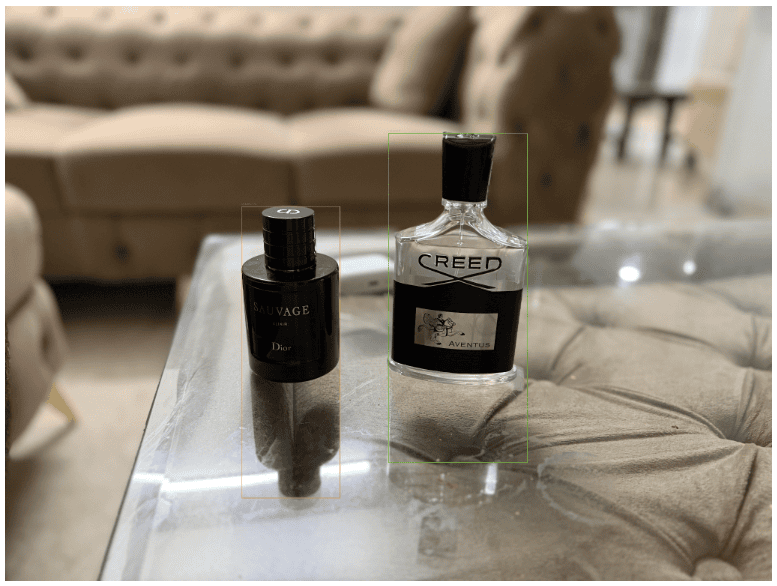
The good news is that YOLOE-26 did most of the tedious work for us.

The bad news is that it did not do all of it.

---

Step 4: Clean the Pseudo-Labels

Raw pseudo-labels are a starting point, not a training set.

That is why scripts/03_clean_pseudo_labels.py applies a second stage of filtering:

def suppress_overlaps(
    detections: list[dict[str, object]],
    min_conf: float,
    iou_threshold: float,
) -> list[dict[str, object]]:
    filtered = [
        detection
        for detection in detections
        if float(detection["confidence"]) >= min_conf
    ]
    filtered.sort(key=lambda item: float(item["confidence"]), reverse=True)

    kept: list[dict[str, object]] = []
    for detection in filtered:
        if any(calculate_iou(detection, existing) >= iou_threshold for existing in kept):
            continue
        kept.append(detection)
    return kept

This script is doing 2 things:

• dropping very weak detections below the confidence threshold
• suppressing weaker overlapping boxes that still survived the earlier consolidation step

We ran it like this:

python3 scripts/03_clean_pseudo_labels.py --split train
python3 scripts/03_clean_pseudo_labels.py --split val

For this project, the cleaned counts ended up like this:

Table 1 already tells an important story. This is a small pilot dataset, not a polished large-scale benchmark setup. We should expect the final fine-tuned detector to be useful, but we should not expect miracles from 41 training images.

What One Cleaned Entry Looks Like

After cleanup and manual correction, a cleaned image entry becomes the record that we trust enough to export:

{
  "image_rel_path": "data/raw/train/session_02_bottle_b_solo/IMG_3858.JPG",
  "preview_image": "data/interim/review_exports/cleaned_predictions/IMG_3858_cleaned_predictions.jpg",
  "detections": [
    {
      "class_id": 1,
      "class_name": "dior_elixir",
      "display_name": "Dior Sauvage Elixir",
      "confidence": 1.0,
      "x1": 1263.0,
      "y1": 2145.0,
      "x2": 2292.0,
      "y2": 3815.0
    }
  ]
}

The following 2 details are worth noticing.

First, the structure is intentionally almost identical to the raw prediction structure. That keeps the manual-fix script simple because it only needs to update the detections list for an image entry instead of rewriting the whole format.

Second, a manual fix can store a confidence of 1.0. That does not mean the detection was magically certain. It means this box was human-approved and should survive the next export step as a trusted label.

The 2 Training Images We Still Had to Fix

Even after cleanup, 2 training images still needed human intervention:

• 1 image had a box that needed to be relabeled from Creed to Dior
• 1 image missed the Dior bottle entirely and needed 1 manual box

That is exactly why scripts/05_manual_fix_cleaned_labels.py exists.

It supports the following 3 edit modes:

• --relabel-only
• --draw-box
• --clear-detections

These were the 2 training fixes we applied:

python3 scripts/05_manual_fix_cleaned_labels.py \
  --split train \
  --image IMG_3859.JPG \
  --class-name dior_elixir \
  --relabel-only

python3 scripts/05_manual_fix_cleaned_labels.py \
  --split train \
  --image IMG_3858.JPG \
  --class-name dior_elixir \
  --draw-box

We also used --clear-detections on true-negative validation images so that empty scenes stayed empty instead of carrying false positives forward.

For example, the helper supports a command like this for a true negative:

python3 scripts/05_manual_fix_cleaned_labels.py \
  --split val \
  --image <IMAGE_NAME> \
  --clear-detections

That tiny branch matters more than it may look. Negative images are one of the easiest ways to teach the final closed-set detector when not to fire.

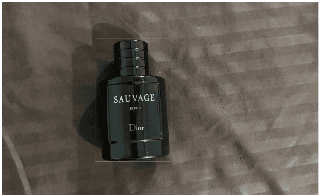
This is the part many pseudo-label tutorials try to glide past. We should not glide past it. The whole point of the workflow is not that the machine makes perfect labels. The point is that it reduces the manual effort to a short correction pass instead of a full box-by-box annotation session.

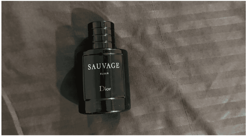
That raw failure is exactly why we do not train directly on pseudo-labels. In this case, a short cleanup pass and 1 manual correction were enough to turn the same image into a usable training example.

---

Step 5: Export the Custom Dataset in Standard YOLO Format

After cleanup, we still need to convert the detections into standard YOLO label files.

That is what scripts/04_export_yolo_dataset.py does.

The core conversion is handled by yolo_line():

def yolo_line(detection: dict[str, object], image_width: int, image_height: int) -> str:
    x1 = float(detection["x1"])
    y1 = float(detection["y1"])
    x2 = float(detection["x2"])
    y2 = float(detection["y2"])
    class_id = int(detection["class_id"])

    box_width = max(0.0, x2 - x1)
    box_height = max(0.0, y2 - y1)
    center_x = x1 + box_width / 2.0
    center_y = y1 + box_height / 2.0

    return " ".join(
        [
            str(class_id),
            f"{center_x / image_width:.6f}",
            f"{center_y / image_height:.6f}",
            f"{box_width / image_width:.6f}",
            f"{box_height / image_height:.6f}",
        ]
    )

This converts corner coordinates into the normalized format (class_id center_x center_y width height) that Ultralytics expects for standard object detection training.

Then the script writes:

• data/processed/yolo_dataset/images/<split>/
• data/processed/yolo_dataset/labels/<split>/
• data/processed/yolo_dataset/data.yaml

Run it like this:

python3 scripts/04_export_yolo_dataset.py --split train
python3 scripts/04_export_yolo_dataset.py --split val

For the train split, the export summary was:

• 41 images
• 50 boxes

At this point, the open-vocabulary stage is done. We now have a standard YOLO detection dataset that required far less manual effort than labeling a dataset from scratch.

What One Exported YOLO Label File Looks Like

Once exported, the label files become plain YOLO detection labels. For example, a label file contains:

1 0.414916 0.521709 0.240196 0.292367

That line contains:

• class ID 1, which configs/classes.yaml maps to dior_elixir
• normalized center x-coordinate: 0.414916
• normalized center y-coordinate: 0.521709
• normalized width: 0.240196
• normalized height: 0.292367

On a pair image, we can have multiple lines:

1 0.373234 0.602377 0.128143 0.507145
0 0.590858 0.507914 0.181373 0.572014

That is the exact point where the open-vocabulary part of the workflow disappears. From here onward, Ultralytics training sees an ordinary 2-class object detection dataset.

---

Step 6: Train YOLO26 on a Custom Dataset

Now we can switch from YOLOE-26 to standard YOLO26 training.

scripts/05_train_yolo26.py wraps the training call and records the main metadata for the run:

train_kwargs = {
    "data": str(dataset_yaml),
    "epochs": args.epochs,
    "imgsz": args.imgsz,
    "batch": args.batch,
    "workers": args.workers,
    "patience": args.patience,
    "project": str(checkpoints_dir),
    "name": args.run_name,
    "seed": args.seed,
    "exist_ok": args.exist_ok,
    "plots": True,
    "val": True,
}

We trained the small (s) checkpoint on Apple Metal Performance Shaders (MPS):

python3 scripts/05_train_yolo26.py \
  --weights yolo26s.pt \
  --epochs 25 \
  --imgsz 960 \
  --batch 8 \
  --patience 8 \
  --device mps

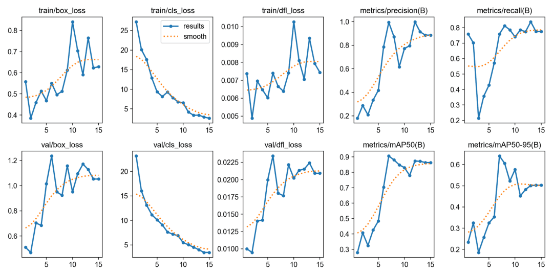
Training stopped early after 15 epochs, and the best checkpoint occurred at epoch 7. Table 2 lists the highest value observed for each validation metric in results.csv:

Mean average precision (mAP) summarizes object detection performance. Mean average precision at an intersection over union (IoU) threshold of 0.50 (mAP50) measures performance at a single threshold. Mean average precision from 0.50 to 0.95 (mAP50-95) averages performance across multiple thresholds.

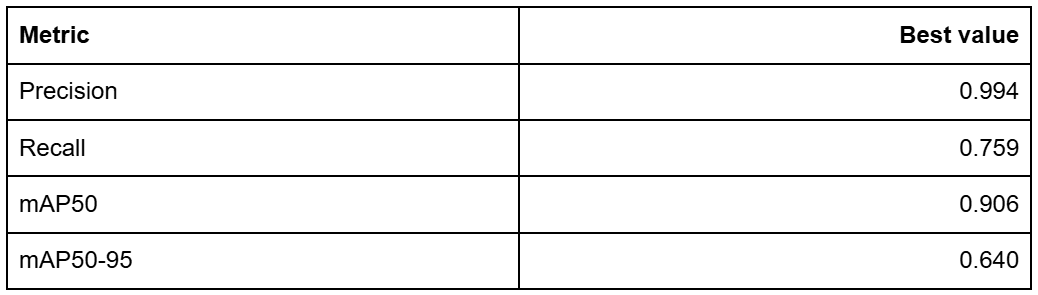
Those are strong numbers for a small 2-class pilot, but we should interpret them carefully. The validation split here is only 9 images with 14 labeled boxes. That means 1 image can change the qualitative story by roughly 11 percentage points at the image level, and 1 missed object can move box recall by about 7 percentage points. The model learned the task well enough to become useful, yet the small data volume still shows up in the qualitative comparisons later, especially on the harder Creed holdout image.

It is also useful to read those numbers with the qualitative results in mind:

• the precision is very high, which matches the fact that the fine-tuned model stays fairly clean on negatives
• the recall is lower, which matches the harder holdout example where Creed is still missed
• the gap between mAP50 and mAP50-95 tells us the detector usually finds the right object, but box quality still has room to tighten up

---

Step 7: Test YOLO26 with Real-Time Webcam Object Detection

Numerical metrics are useful, but they do not tell the whole story for a small custom detector.

That is why we added scripts/06_webcam_demo.py.

The script loads the fine-tuned checkpoint, runs live inference on webcam frames, and overlays the current class counts:

result = model.predict(
    source=frame,
    conf=args.conf,
    imgsz=args.imgsz,
    verbose=False,
)[0]
annotated = result.plot()

Run it like this:

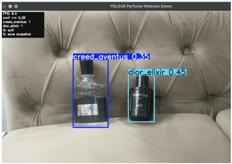
python3 scripts/06_webcam_demo.py --conf 0.35 --device mps

One practical lesson from our pilot run is that the webcam threshold needed to stay fairly low. Around 0.35, the detector recognized both bottles reliably. Pushing the threshold much higher made detections disappear too aggressively.

That does not mean the model is broken. It means we trained on a small, narrow dataset and should treat the confidence threshold as a tunable deployment parameter, not as a universal fixed value. In small custom detectors, a threshold of 0.35 can be perfectly reasonable if it matches the behavior we want on real scenes.

Another useful way to frame it is this: the webcam demo is not a benchmark. It is a human-in-the-loop product check. If 0.35 gives us the detections we actually want on live camera frames, that is a valid operating point for this pilot. We would only raise it once we had enough additional data to do so without collapsing recall.

---

Step 8: Compare YOLO26, YOLOE-26, and Fine-Tuned Object Detection Models

The last script, scripts/07_evaluate_models.py, creates the side-by-side figures that make the whole lesson defensible.

For each validation image, it renders:

• the original image
• the baseline closed-set YOLO26 result
• the YOLOE-26 visual-prompt result
• the fine-tuned YOLO26 result

Run it like this:

python3 scripts/07_evaluate_models.py --split val --device mps

The script writes the final comparison panels to outputs/figures/comparison_val/.

This is where the story gets interesting, because the answer is not simply “the fine-tuned model wins everywhere.”

What the Evaluation Script Is Doing Behind the Scenes

The comparison script is worth a little extra attention because it does more than call predict() for each of the 3 detectors.

For the fine-tuned YOLO26 result, we first convert the Ultralytics result object into a simple list of rows, suppress overlapping duplicates, and then rebuild a filtered result object before plotting:

finetuned_rows = consolidate_image_detections(yolo_result_to_rows(finetuned_result))
finetuned_filtered_result = clone_result_with_rows(finetuned_result, finetuned_rows)
finetuned_tile = finetuned_filtered_result.plot(conf=False)

That step ended up mattering for exactly the kind of issue we saw in IMG_3885, where near-identical duplicate boxes can clutter a final figure even if the underlying prediction is basically correct.

The script also removes confidence text from the baseline and fine-tuned comparison panels. That was the right editorial choice here, because a YOLOE-26 confidence value and a fine-tuned YOLO26 confidence value are not directly comparable on one shared scale.

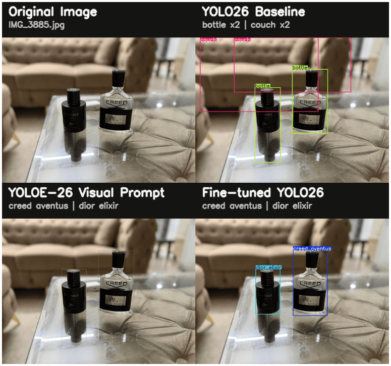
Case 1: A Clean Success Example

On IMG_3885, the comparison is exactly what we hoped for:

• baseline YOLO26 sees generic bottles and extra furniture classes
• YOLOE-26 visual prompting finds both custom bottles
• the fine-tuned YOLO26 detector also finds both custom bottles

This is the strongest example to show the workflow working end to end.

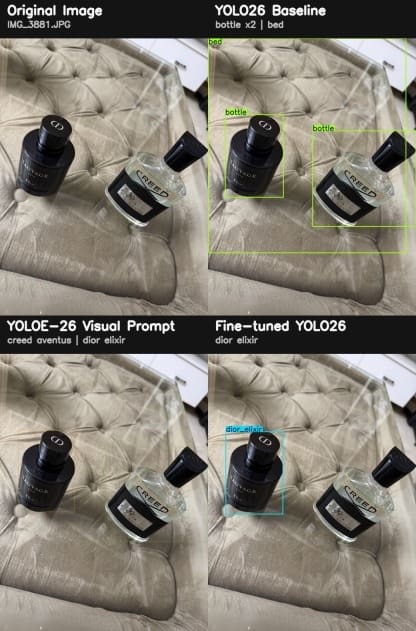
Case 2: A Harder Holdout Where the Fine-Tuned Detector Still Misses Creed

On IMG_3881, the story changes:

• baseline YOLO26 still sees only generic bottle-like objects
• YOLOE-26 visual prompting still finds both target classes
• the fine-tuned YOLO26 detector finds Dior but misses Creed

This is not a failure of the lesson. It is an honest reminder that 41 training images are enough to build a meaningful pilot, but not enough to erase every weak spot immediately.

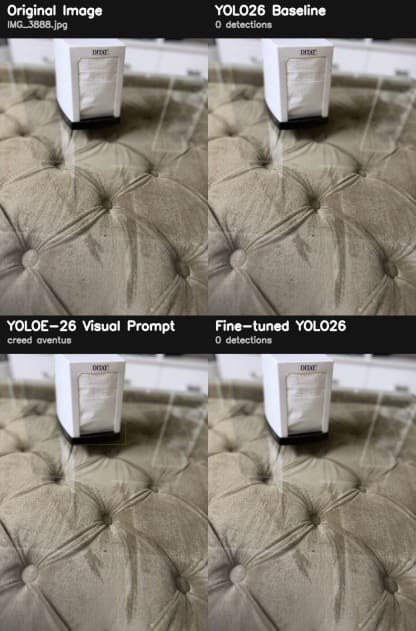
Case 3: A Negative Image Where the Fine-Tuned Detector Stays Clean

On IMG_3888, the comparison tells a different kind of story:

• baseline YOLO26 predicts nothing
• YOLOE-26 visual prompting produces a false positive
• the fine-tuned YOLO26 detector predicts nothing

This is a useful reminder that open-vocabulary prompting and closed-set specialization have different failure modes. YOLOE-26 is the better search tool. The fine-tuned YOLO26 model can be the cleaner deployment artifact once the class list is stable.

---

Why Fine-Tune YOLO26 If YOLOE-26 Already Works?

This is the right question to ask, especially after looking at the comparison figures.

In our pilot, YOLOE-26 visual prompting is often the strongest approach in terms of raw recall. It also tends to assign higher confidence scores to those detections.

That does not make the fine-tuning step pointless.

Here is the practical framing:

• YOLOE-26 is the discovery and bootstrapping tool.
• Fine-tuned YOLO26 is the deployment candidate for a stable label set.

There are 4 reasons that distinction still matters.

Prompt Setup Disappears at Inference Time

The fine-tuned YOLO26 model does not need prompt boxes, reference images, or prompt management logic. We just load the checkpoint and run inference.

The Artifact Is Narrower and Easier to Reason About

Once the class list is fixed, a 2-class closed-set detector is simpler to package, explain, and maintain than a prompt-driven open-vocabulary workflow.

It Can Get Cleaner as Corrected Data Accumulates

The current pilot used 41 training images. If we keep correcting labels and adding more scenes, the fine-tuned detector should get better exactly where it is weakest today.

Confidence Values Are Not Directly Comparable Across the 2 Models

This point matters a lot. A 0.90 score from YOLOE-26 and a 0.45 score from the fine-tuned YOLO26 model are not the same kind of number. They come from different training setups and different decision surfaces. We should compare them by behavior on held-out images, not by treating the raw confidence values as if they lived on one universal scale.

So the right takeaway is not “fine-tuning instantly beats YOLOE-26.” The right takeaway is:

YOLOE-26 helped us create a usable class-specific detector far faster than a manual labeling workflow would have.

---

What This Workflow Covered and What It Did Not

In this lesson, we covered the entire practical pipeline:

• class configuration
• reference prompt selection
• visual-prompt pseudo-labeling
• confidence cleanup
• manual patching of edge cases
• YOLO-format export
• fine-tuning
• webcam inference
• qualitative comparison

What we did not cover is equally important:

• we did not train YOLOE-26 itself
• we did not build a large-scale benchmark
• we did not prove that 41 images are enough for a production-ready custom detector in every setting

This was a pilot workflow, and it succeeded as a pilot workflow. It gave us a fast, credible way to move from open-vocabulary search to a real fine-tuned detector on our own classes.

---

---

Summary

Lesson 1 showed how YOLOE-26 expands YOLO into the open-vocabulary world.

Lesson 2 showed why that matters in practice.

We used YOLOE-26 visual prompting to auto-label a small custom dataset, cleaned the noisy predictions, fixed the few images that still needed human help, exported the result into standard YOLO format, and fine-tuned yolo26s.pt into a 2-class perfume detector that we could run both on validation images and in a live webcam demo.

The most important result is not a single metric. It is the workflow itself.

Instead of starting with unlabeled data and creating every annotation by hand, we used open-vocabulary detection as the first draft of a custom training set. That is the bridge between flexible promptable detection and a simpler deployment model.

If we wanted to keep going from here, the next improvements would be obvious:

• collect more Creed-heavy training views
• add more negative scenes
• add more cluttered backgrounds
• rerun the exact same pipeline

That is a good sign. It means we do not need a different system. We just need to process more corrected data through the same pipeline.

Citation Information

Singh, V. “Train YOLO26 on a Custom Dataset with YOLOE-26 Auto-Labeling,” PyImageSearch, S. Huot, A. Sharma, and P. Thakur, eds., 2026, https://pyimg.co/xrtzy

@incollection{Singh_2026_train-yolo26-custom-dataset-yoloe-26-auto-labeling,
  author = {Vikram Singh},
  title = {{Train YOLO26 on a Custom Dataset with YOLOE-26 Auto-Labeling}},
  booktitle = {PyImageSearch},
  editor = {Susan Huot and Aditya Sharma and Piyush Thakur},
  year = {2026},
  url = {https://pyimg.co/xrtzy},
}

---

To download the source code to this post (and be notified when future tutorials are published here on PyImageSearch), simply enter your email address in the form below!