CycleGAN: Unpaired Image-to-Image Translation (Part 2)

---

Table of Contents

---

CycleGAN: Unpaired Image-to-Image Translation (Part 2)

In this tutorial, we will implement our CycleGAN model for unpaired image-to-image translation tasks using TensorFlow and Keras. We will dive into the details of the CycleGAN model architecture and discuss the Apples2Oranges Dataset, which we will use for our unpaired image translation task.

This lesson is the 2nd in a 3-part series on GANs 301:

1. CycleGAN: Unpaired Image-to-Image Translation (Part 1)
2. CycleGAN: Unpaired Image-to-Image Translation (Part 2) (this tutorial)
3. CycleGAN: Unpaired Image-to-Image Translation (Part 3)

To learn how to implement CycleGAN for Unpaired Image-to-Image Translation, just keep reading.

---

CycleGAN: Unpaired Image-to-Image Translation (Part 2)

In the previous tutorial of this series, we discussed the task of unpaired image-to-image translation and got a high-level intuition of the CycleGAN model. Furthermore, we delved deeper into the mechanism and loss functions used by CycleGAN to seamlessly perform image-to-image translations from a dataset of unpaired images.

In this tutorial, we will continue our discussion and implement the architecture of our CycleGAN model from scratch using Keras and TensorFlow. Furthermore, we look closer at the Apples2Oranges Dataset and discuss dataset preprocessing techniques, allowing us to process our input data and build our end-to-end image translation model.

---

Apples2Oranges Dataset

As discussed briefly in the previous tutorial of this series, we will be using the Apples2Oranges Dataset in this tutorial to perform image translation. The Apples2Oranges Dataset was officially introduced in Unpaired Image-to-Image Translation Using Cycle-Consistent Adversarial Networks. It was used to show the unpaired image-to-image translation performance and capabilities of CycleGAN. It can be easily found and downloaded from Roboflow.

We can easily download and get quick access to this dataset from Roboflow universe Apples2Oranges Dataset section. Roboflow provides easy and quick access to many curated computer vision datasets for diverse tasks like Single or Multi-Label Classification, Object Detection, Instance Segmentation etc. It also provides an amazing API that seamlessly allows you to upload your own datasets and apply data augmentation techniques and transformations on your images in real-time. 

If you are interested in experiencing the amazing Roboflow universe and the features it provides quickly head over to the Roboflow website and get your free account now. Go ahead and get started with the tutorials which will help you get started and fully enjoy the features of the roboflow universe.

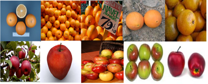
This dataset consists of 1261 Apples’ Photos & 1267 Oranges’ Photos which form the two domains between which image translation is performed. Notice that the dataset consists of approximately equal numbers of apple and orange data samples.

Furthermore, the dataset is split into a train set which consists of 80% of the data, and a test set which consists of 20% of the data. Figure 1 shows some example images for apples (bottom) and oranges (top) from this dataset.

---

Configuring Your Development Environment

To follow this guide, you need to have the TensorFlow library installed on your system.

Luckily, TensorFlow is pip-installable:

$ pip install tensorflow

---

Need Help Configuring Your Development Environment?

All that said, are you:

• Short on time?
• Learning on your employer’s administratively locked system?
• Wanting to skip the hassle of fighting with the command line, package managers, and virtual environments?
• Ready to run the code now on your Windows, macOS, or Linux system?

Then join PyImageSearch University today!

Gain access to Jupyter Notebooks for this tutorial and other PyImageSearch guides that are pre-configured to run on Google Colab’s ecosystem right in your web browser! No installation required.

And best of all, these Jupyter Notebooks will run on Windows, macOS, and Linux!

---

Project Structure

We first need to review our project directory structure.

Start by accessing this tutorial’s “Downloads” section to retrieve the source code and example images.

From there, let us take a look at the directory structure:

├── inference.py
├── outputs
│   ├── images
│   └── models/generator
├── pyimagesearch
│   ├── CycleGANTraining.py
│   ├── __init__.py
│   ├── config.py
│   ├── data_preprocess.py
│   ├── model.py
│   └── train_monitor.py
└── train.py

The inference.py file implements the code we will use during the inference stage to translate images in real-time and see our model in action. Finally, the outputs folder is where we store the output images and save our trained CycleGAN model.

The pyimagesearch folder contains the main components of our CycleGAN pipeline. In addition, this folder includes the CycleGANTraining.py file, which implements the training procedure for our model.

Furthermore, the config.py file contains the parameter configurations we will use while implementing our image translation pipeline, and the data_preprocess.py file contains the dataset preprocessing code.

The model.py file implements the architecture of our CycleGAN model, and the train_monitor.py file implements a callback which will allow us to visualize and monitor the training process.

Finally, the train.py file implements the code to train our end-to-end CycleGAN model.

In this part, we will discuss the config file, the implementation of the model architecture (i.e., model.py file), and the data preprocess procedure (i.e., data_preprocess.py file).

In the next part of this blog series, we will dive deeper into the training process of our image translation model. Specifically, we will discuss the CycleGANTraining.py and train.py files along with the callback implementation, which will help us monitor the training process (i.e., the train_monitor.py file). Furthermore, we will also look into the inference stage of our trained CycleGAN model and discuss the inference.py file in detail.

---

Creating Our Configuration File

We start by opening the config.py file, which contains the parameters and initial configurations we will use to implement our CycleGAN model.

# import the necessary packages
import os

# define the batch size for training and inference
TRAIN_BATCH_SIZE = 1
INFER_BATCH_SIZE = 8

# dataset specs
IMG_WIDTH = 256
IMG_HEIGHT = 256
IMG_CHANNELS = 3

# training specs
LR = 2e-4
EPOCHS = 50
STEPS_PER_EPOCH = 800

# path to the base output directory
BASE_OUTPUT_PATH = "outputs"

# path to the cycle gan generator
GENERATOR_MODEL = os.path.join(BASE_OUTPUT_PATH, "models",
    "generator")

# path to the inferred images and to the grid image
BASE_IMAGES_PATH = os.path.join(BASE_OUTPUT_PATH, "images")
GRID_IMAGE_PATH = os.path.join(BASE_IMAGES_PATH, "grid.png")

On Line 2, we import the os module for file system functionalities. Next, we define our batch size for training (i.e., TRAIN_BATCH_SIZE) and inference stage (i.e., INFER_BATCH_SIZE) on Lines 5 and 6, respectively.

Next, we define our data parameters, such as the dimensions (i.e., IMG_WIDTH and IMG_HEIGHT) of the image and the number of channels (i.e., IMG_CHANNELS) (Lines 9-11).

Furthermore, we define the specifications for our training process, such as the learning rate (i.e., LR), the total number of epochs (i.e., EPOCHS), and the number of iterations or steps per epoch (i.e., STEPS_PER_EPOCH), as shown on Lines 14-16.

On Line 19, we define the parent output directory (i.e., BASE_OUTPUT_PATH), and on Line 22, we define the path where the CycleGAN generator will be saved after training (i.e., GENERATOR_MODEL).

Finally, we define the paths where our visualizations from the inference stage will be stored (i.e., BASE_IMAGES_PATH and GRID_IMAGE_PATH) on Lines 26 and 27.

---

Preprocessing Our Dataset

Now that we have discussed the config file and defined the initial parameter configurations, we are ready to discuss the code that will allow us to preprocess our input data during the training and testing or inference stage.

We open the data_preprocess.py file, which implements this code, and start.

# import the necessary packages
import tensorflow as tf

def preprocess_image(image):
    # convert both images to float32 tensors and
    # convert pixels to the range of -1 and 1
    image = tf.cast(image, tf.float32) / 127.5 - 1

    # return the image
    return (image)
    
def random_jitter(image):
    # upscale the image and randomly crop them
    image = tf.image.resize(image, [286, 286],
        method=tf.image.ResizeMethod.NEAREST_NEIGHBOR)
    cropped = tf.image.random_crop(image, size=[256, 256, 3])

    # randomly flip the cropped image
    image = tf.image.random_flip_left_right(cropped)

    # return the image
    return image

def read_train_example(data):
    # pre-process the image
    image = preprocess_image(data["image"])
    image = random_jitter(image)

    # reshape the input image
    image = tf.image.resize(image, [256, 256])

    # return the input image
    return (image)

def read_test_example(data):
    # pre-process the image and resize it
    image = preprocess_image(data["image"])
    image = tf.image.resize(image, [256, 256])

    # return the image
    return (image)

We start by importing the tensorflow library on Line 2.

Next, on Lines 4-10, we write the preprocess_image() function, which will allow us to preprocess our images. The function takes the image as input to pre-process, as shown on Line 4.

Then, on Line 7, we convert the image to tf.float32 format using the tf.cast() function and convert its pixels to the range [-1,1]. Since the pixel values are in the range [0,255], we can achieve this by dividing the pixel values by 127.5 and subtracting the value 1. Finally, we return the pre-processed image on Line 10.

Then, on Lines 12-22, we define the random_jitter() function, which will apply data augmentations to our input images. The function takes the image as input to apply data augmentations, as shown on Line 12. Next, on Line 14, we use the tf.image.resize() function to upscale the image to the [286,286] size using the NEAREST_NEIGHBOR interpolation technique, as shown.

Then, on Line 16, we randomly crop the image to the desired size [256, 256, 3] using the tf.image.random_crop function. Finally, we use the tf.image.random_flip_left_right() function on our upscaled and cropped image to apply random flip augmentation and return our final output image on Line 22.

On Lines 24-33, we define the read_train_example() function, which takes as input the data and allows us to apply pre-processing and data augmentation operations to our data during training. Next, we use the preprocess_image() function and the random_jitter() function we defined above on Lines 26 and 27, respectively. Then, on Line 30, we resize our image to the desired [256, 256] dimension and finally return our image on Line 33.

Similar to the read_train_example() function, we now define the read_test_example function, which allows us to pre-process our data during test time. However, since we need to apply data augmentations only during training and not during test time, we only pre-process our image using the preprocess_image function on Line 37 and resize our image to the desired [256, 256] dimension and finally return our image on Line 41.

---

Implementing the CycleGAN Architecture

We are now ready to dive into the details of our CycleGAN architecture and implement it from scratch using Keras and TensorFlow.

As discussed in the first part of this series, the CycleGAN model consists of two generators and two discriminators. We will create a CycleGAN class that implements our generator architecture and discriminator architecture.

Note that the generator of our CycleGAN follows a structure similar to U-Net with a succession of downsampling layers, the U-shaped bend followed by a succession of upsampling layers with skip connections.

If you are unfamiliar with the U-Net architecture or wish to brush up on the concepts, we have an amazing tutorial that offers an in-depth explanation of the U-Net architecture (U-Net: Training Image Segmentation Models in PyTorch).

We open the model.py file containing the code to implement our CycleGAN model definition and get started.

# import the necessary packages
from tensorflow.keras.layers import BatchNormalization
from tensorflow.keras.layers import Conv2DTranspose
from tensorflow.keras.layers import LeakyReLU
from tensorflow.keras.layers import concatenate
from tensorflow.keras.layers import MaxPool2D
from tensorflow.keras.layers import Conv2D
from tensorflow.keras.layers import Dropout
from tensorflow.keras import Model
from tensorflow.keras import Input

class CycleGAN():
    def __init__(self, imageHeight, imageWidth):
        # initialize the image height and width
        self.imageHeight = imageHeight
        self.imageWidth = imageWidth

    def generator(self):
        # initialize the input layer
        inputs = Input([self.imageHeight, self.imageWidth, 3])
  
        # down Layer 1 (d1) => final layer 1 (f1)
        d1 = Conv2D(32, (3, 3), activation="relu", padding="same")(
            inputs)
        d1 = Dropout(0.1)(d1)
        f1 = MaxPool2D((2, 2))(d1)

        # down Layer 2 (l2) => final layer 2 (f2)
        d2 = Conv2D(64, (3, 3), activation="relu", padding="same")(f1)
        f2 = MaxPool2D((2, 2))(d2)

        #  down Layer 3 (l3) => final layer 3 (f3)
        d3 = Conv2D(96, (3, 3), activation="relu", padding="same")(f2)
        f3 = MaxPool2D((2, 2))(d3)

        # down Layer 4 (l3) => final layer 4 (f4)
        d4 = Conv2D(96, (3, 3), activation="relu", padding="same")(f3)
        f4 = MaxPool2D((2, 2))(d4)

        # u-bend of the u-bet
        b5 = Conv2D(96, (3, 3), activation="relu", padding="same")(f4)
        b5 = Dropout(0.3)(b5)
        b5 = Conv2D(256, (3, 3), activation="relu", padding="same")(b5)

        # upsample Layer 6 (u6)
        u6 = Conv2DTranspose(128, (2, 2), strides=(2, 2),
            padding="same")(b5)
        u6 = concatenate([u6, d4])
        u6 = Conv2D(128, (3, 3), activation="relu", padding="same")(
            u6)

        # upsample Layer 7 (u7)
        u7 = Conv2DTranspose(96, (2, 2), strides=(2, 2),
            padding="same")(u6)
        u7 = concatenate([u7, d3])
        u7 = Conv2D(128, (3, 3), activation="relu", padding="same")(
            u7)

        # upsample Layer 8 (u8)
        u8 = Conv2DTranspose(64, (2, 2), strides=(2, 2),
            padding="same")(u7)
        u8 = concatenate([u8, d2])
        u8 = Conv2D(128, (3, 3), activation="relu", padding="same")(u8)

        # upsample Layer 9 (u9)
        u9 = Conv2DTranspose(32, (2, 2), strides=(2, 2),
            padding="same")(u8)
        u9 = concatenate([u9, d1])
        u9 = Dropout(0.1)(u9)
        u9 = Conv2D(128, (3, 3), activation="relu", padding="same")(u9)

        # final conv2D layer
        outputLayer = Conv2D(3, (1, 1), activation="tanh")(u9)
    
        # create the generator model
        generator = Model(inputs, outputLayer)

        # return the generator
        return generator

We start by importing the important layers to help us build our CycleGAN model on Lines 2-10. Then, on Lines 12-79, we define our CycleGAN() class.

We start by defining the __init__ constructor first (Lines 13-16), which takes as input the imageHeight and imageWidth as shown on Line 13 and initializes the self.imageHeight and self.imageWidth attributes of the class on Lines 15 and 16.

Next, on Lines 18-79, we implement the definition of our CycleGAN generator. We start by initializing the Input layer with the desired dimensions of our input, which is [self.imageHeight, self.imageWidth, 3] on Line 20. Then we begin downsampling our input with a sequence of Conv2D → Dropout → MaxPool2D layers, as shown on Lines 23-26. We further downsample using a sequence of Conv2D → MaxPool2D operations as shown on Lines 29-38.

Then we build the U-shaped bend of our generator using a Conv2D → Dropout → Conv2D sequence of layers, as shown on Lines 41-43, and finally, we use a succession of Conv2DTranspose → concatenate → Conv2D layers to upsample our feature maps, as shown on Lines 46-70.

Note that the concatenate operation implements the skip connections of the U-Net by concatenating the features from the downsampling part of the U shape to the upsampling part of the U shape.

Finally, we have our 1×1 Conv2D output layer (Line 73). We create our generator model using the Model functionality of Keras with the inputs and outputLayer layers as the input and output of our generator model. We then return our generator model on Line 79.

   def discriminator(self):
        # initialize input layer according to PatchGAN
        targetImage = Input(
            shape=[self.imageHeight, self.imageWidth, 3], 
            name="target_image"
        )

        # add four conv2D convolution layers
        x = Conv2D(64, 4, strides=2, padding="same")(targetImage)  
        x = LeakyReLU()(x)
        x = Conv2D(128, 4, strides=2, padding="same")(x)
        x = LeakyReLU()(x)  
        x = Conv2D(256, 4, strides=2, padding="same")(x)
        x = LeakyReLU()(x)   
        x = Conv2D(512, 4, strides=1, padding="same")(x)  

        # add a batch-normalization layer => LeakyReLU => zeropad
        x = BatchNormalization()(x)
        x = LeakyReLU()(x)

        # final conv layer
        last = Conv2D(1, 3, strides=1)(x) 
  
        # create the discriminator model
        discriminator = Model(inputs=[targetImage],
            outputs=last)

        # return the discriminator
        return discriminator

Now that we have defined our generator, we are ready to define the discriminator of our CycleGAN (Lines 81-109). We initialize the input layer using the Input functionality with shape [self.imageHeight, self.imageWidth, 3] and layer name as target_image.

Then we use a succession of Conv2D → LeakyReLU layers, as shown on Lines 89-95, to build our discriminator. We then add a BatchNormalization layer → LeakyReLU sequence (Lines 98 and 99) and finally use a Conv2D layer as the last layer of our discriminator (Line 102).

Similar to what we did in the generator case, we then create our discriminator model using the Model functionality of Keras with the [targetImage] and last layer as the model input and output (Lines 105 and 106). We then return our discriminator model on Line 109.

This completes the implementation of our CycleGAN model, which consists of the generator and discriminator architectures, as discussed in detail above.

---

---

Summary

In this tutorial, we continued our discussion on CycleGAN and unpaired image-to-image translation, which we started in the previous post of this series.

Specifically, we implemented the CycleGAN architecture in Keras and TensorFlow from scratch. We implemented the code to pre-process our input data during the training and testing stages of our CycleGAN pipeline.

In the next tutorial of this series, we will dive deeper into the training and inference details of our CycleGAN and see how we can use it to perform the unpaired image-to-image translation in real-time.

---

Citation Information

Chandhok, S. “CycleGAN: Unpaired Image-to-Image Translation (Part 2),” PyImageSearch, P. Chugh, A. R. Gosthipaty, S. Huot, K. Kidriavsteva, R. Raha, and A. Thanki, eds., 2023, https://pyimg.co/jnael

@incollection{Chandhok_2023_CycleGAN-Part2,
  author = {Shivam Chandhok},
  title = {{CycleGAN}: Unpaired Image-to-Image Translation (Part 2)},
  booktitle = {PyImageSearch},
  editor = {Puneet Chugh and Aritra Roy Gosthipaty and Susan Huot and Kseniia Kidriavsteva and Ritwik Raha and Abhishek Thanki},
  year = {2023},
  url = {https://pyimg.co/jnael},
}

---

---

To download the source code to this post (and be notified when future tutorials are published here on PyImageSearch), simply enter your email address in the form below!