Diagonalize Matrix for Data Compression with Singular Value Decomposition

Matrix decomposition is a fundamental concept in linear algebra that simplifies complex matrix operations, making them more manageable and revealing the underlying structure of data. Singular Value Decomposition (SVD) is one of the most powerful matrix decomposition techniques. It breaks down a matrix into three simpler matrices, allowing us to analyze the original data more efficiently.

SVD has significant applications in data compression, where it reduces the size of data while preserving its essential information. Using SVD for data compression involves transforming the data matrix into a diagonal form consisting of singular values. By retaining only the largest singular values, we can significantly reduce the data size while preserving essential details and discarding redundant information.

This process helps in compressing data, making storage and transmission more efficient. In this blog post, we will understand the concept of SVD and know how it can be used for matrix diagonalization and data compression.

This lesson is the 2nd of a 3-part series on Matrix Factorization:

Solving System of Linear Equations with LU Decomposition
Diagonalize Matrix for Data Compression with Singular Value Decomposition (this tutorial)
Solving System of Linear Equations with QR Decomposition

To learn how to diagonalize a matrix with singular value decomposition, just keep reading.

Looking for the source code to this post?

What Is Matrix Diagonalization?

Matrix diagonalization is a process in linear algebra where a given matrix is transformed into a diagonal matrix. A diagonal matrix is a special type of matrix where all the off-diagonal elements are zero, and the diagonal elements capture the essential characteristics of the original matrix. Diagonalization simplifies many matrix operations and provides deeper insights into the properties of the matrix.

Mathematical Definition

In an $m \times n$ matrix, $A$ can be diagonalized and expressed in the following form:

$A = PDQ^T$

where:

$P$ is an $m \times r$ orthogonal matrix (i.e., $PP^T = I$ )
$D$ is an $r \times r$ diagonal matrix whose diagonal elements are non-negative real numbers (known as singular values).
$Q$ is an $n \times r$ orthogonal matrix (i.e., $QQ^T = I$ )

Figure 1 shows how a matrix $M$ can be decomposed into a product of two orthogonal matrices ( $U$ and $V$ ) and one diagonal matrix ( $D$ ).

**Figure 1:** General form of Matrix Diagonalization (source: Math3ma).

Singular Value Decomposition

Singular Value Decomposition (SVD) is a popular algorithm used to diagonalize a matrix of an arbitrary $m \times n$ shape. SVD splits any matrix $A$ into three simpler matrices: $U$ , $\Sigma$ , and $V^T$ (Figure 2):

$A = U \Sigma V^T$

where $U$ and $V$ are orthogonal matrices known as left and right singular matrices, and $\Sigma$ is an $r \times r$ diagonal matrix containing the singular values. These values are typically sorted in descending order:

$\sigma_1 \geq \sigma_2 \geq \ldots \geq \sigma_r \geq 0$

where $r = \min(m, n)$ .

**Figure 2:** Singular Value Decomposition (SVD) (source: AskPython).

How to Diagonalize Matrix with Singular Value Decomposition

The Power Iteration method is a simple and efficient algorithm for finding the largest singular values and corresponding singular vectors of a matrix 1×1 in an iterative fashion. It involves repeatedly multiplying a random vector by the matrix until convergence.

Power Iteration Algorithm

Given a matrix $A$ of size $m \times n$ , the power iteration algorithm to obtain $U$ , $\Sigma$ , and $V^T$ involves the following steps.

Step 1: Start with a Random Vector

Start with a random vector $x_0 \in \mathbb{R}^n$ of size $n$ .

Step 2: Iteratively Refine the Vector

Apply the power iteration method to refine $w_0$ (Figure 3) and approximate the largest singular value:

$w_{k+1} = \displaystyle\frac{A^TA w_k}{\vert A w_k \vert}$

$\sigma_1 \approx \vert A^T w_k \vert$

where $\vert . \vert$ is the Euclidean norm of the vector. Repeat this process until convergence.

**Figure 3:** Power iteration method keeps refining vector $w_k$ (source: Gaston Sanchez).

Step 3: Construct the Singular Vectors

Once we have the largest singular value $\sigma_1$ and its corresponding singular vector $w$ , we can compute the first column of matrices $U$ and $V$ as follows:

The Right Singular Vector $v_1$ is given as $v_1 = \displaystyle\frac{w}{\vert w \vert}$
The Left Singular Vector $u_1$ is given as $u_1 = \displaystyle\frac{A v_1}{\sigma_1}$

Step 4: Deflate the Matrix

To find other singular values and vectors, we need to update the matrix $A$ as follows:

$A^\prime = A - \sigma_1 u_1 v_1^T$

Once we have the updated matrix, we can apply the power iteration method again (i.e., repeat from Step 1) on the updated matrix $A^\prime$ to find the next singular value $\sigma_2$ and its corresponding singular vectors.

Step 5: Form the Matrices U, Σ, and V

We can repeat the above steps until we have all the $r = \min(m, n)$ singular values $\sigma_1 \geq \sigma_2 \geq \ldots \geq \sigma_r \geq 0$ and their corresponding left and right singular vectors.

Next, we form the matrices $U$ , $\Sigma$ , and $V$ :

Matrix $U$ : The columns of $U$ are the left singular vectors $u_i$ .
Matrix $\Sigma$ : The diagonal elements of $\Sigma$ are the singular values $\sigma_i$ .
Matrix $V$ : The columns of $V$ are the right singular vectors $v_i$ .

Calculating SVD Using Power Iteration

The following code snippet calculates the Singular Value Decomposition of a matrix using the power iteration method described above. The code uses the NumPy library, which can be installed in your Python environment via pip install numpy.

import numpy as np

def power_iteration(A, num_iter=50000, tol=1e-6):
   
    m, n = A.shape[0], A.shape[1]
    r = min(m, n)
    U, Sigma, V = [], [],  []

On Lines 1-7, we import the necessary library, define the power_iteration function, and initialize key variables such as the dimensions of A, and empty lists to store the singular vectors and values. We also set the number of iterations and tolerance for convergence.

    for i in range(r):
      B = A.T.dot(A)

      # Step 1: Define random vector
      x = np.random.rand(n)

      # Step 2: Iteratively Refine the Vector
      for _ in range(num_iter):
        Bx = np.dot(B, x)
        x_new = Bx / np.linalg.norm(Bx)

        # Check for convergence
        if np.linalg.norm(x_new - x) < tol:
            break

      # Step 3: Construct the Singular Vectors
      x = x_new
      v = x / np.linalg.norm(x)
      s = np.linalg.norm(np.dot(A, v))
      u = np.dot(A, x)/s
     

      U.append(u)
      Sigma.append(s)
      V.append(v)

      # Step 4: Deflate the Matrix and Repeat
      A = A - s * np.outer(u, v)

    # Step 5: Form the Matrices U, Σ, and V
    return np.array(U).T, np.diag(Sigma), np.array(V).T

On Lines 9-39, we use a for-loop to iterate through the possible singular values (up to rank r). Inside this loop, we first compute B as (A.T)A (Line 10). Next, we initialize a random vector x (Line 13) and iteratively refine it using the power iteration method (Lines 16-22).

After convergence, we normalize the vector to form the right singular vector v, calculate the corresponding singular value s, and compute the left singular vector u (Lines 25-33). These values are appended to their respective lists, and the matrix A is deflated to remove the contribution of the computed singular value (Line 36). On Line 39, we form the matrices U, Σ, and V from the computed singular vectors and values and return them.

# Example usage
A = np.array([[1, 2], [3, 4], [5, 6]]) # 3 x 2 matrix
U, S, VT = power_iteration(A.copy())
print("Left Singular Matrix U: \n", U)
print("Singular Values S: \n", S)
print("Right Singular Matrix VT: \n", VT)

print("Verifying A = U S V^T \n", U.dot(S).dot(VT))

Finally, in the example usage (Lines 42-48), we define a matrix A, apply the power_iteration function, and print the resulting matrices to verify the decomposition. This step-by-step approach demonstrates how the Power Iteration method can be used to approximate SVD without relying on advanced library functions.

Output:

Left Singular Matrix U: 
 [[ 0.22977391 -0.88968133]
 [ 0.52472471 -0.25571211]
 [ 0.81967551  0.37825712]]

Singular Values S: 
 [[9.52550673 0.        ]
 [0.         0.51451101]]

Right Singular Matrix VT: 
 [[ 0.62084292  0.78393499]
 [ 0.78393499 -0.62084292]]

Verifying A = U S V^T 
 [[1. 2.]
 [3. 4.]
 [5. 6.]]

Data Compression Using Singular Value Decomposition

Using Diagonalizable Matrix for Data Compression

Using diagonalizable matrices for data compression involves leveraging the properties of matrices that can be expressed in a diagonal form to reduce the amount of data stored or transmitted. This method capitalizes on the fact that diagonalized matrices often contain redundant or less significant information that can be discarded without severely impacting the quality of the data.

The key to data compression lies in the singular values. During a Singular Value Decomposition, these singular values are ordered in descending magnitude in $\Sigma$ , with the most significant ones appearing first.

$\sigma_1 \geq \sigma_2 \geq \ldots \geq \sigma_r \geq 0$

The largest singular values represent the directions in which the data exhibits the most variance. These values capture the most significant features of the data, whereas the smallest singular values indicate directions with less variance, often representing noise or less critical components of the data (Figure 4).

**Figure 4:** Visualization of singular values (source: Wikipedia).

As can be seen in Figure 4, the largest singular value ( $\sigma_1$ ) represents the direction with the most variance, whereas the smallest singular value ( $\sigma_2$ ) indicates the direction with the least variance.

In many practical scenarios, only a few of these large singular values are necessary to capture the essential features of the data. By truncating the less significant smaller singular values, we can approximate the original matrix with a lower rank, thereby reducing its size. In other words:

Decompose the Matrix: Perform SVD on the original matrix $A$ to obtain $U$ , $\Sigma$ , and $V^T$ .
Truncate the Singular Values: Identify a threshold and retain only the top $k$ singular values in $\Sigma$ , along with the corresponding columns in $U$ and $V^T$ . The truncated matrices are denoted as $U_k$ , $\Sigma_k$ , and $V_k^T$ (Figure 5).
Reconstruct the Matrix: Approximate the original matrix $A$ using the truncated matrices: $A \approx A_k = U_k \Sigma_k V_k^T$

This results in a lower-rank approximation $A_k$ — a compressed version of the original matrix $A$ .

**Figure 5:** Truncated SVD for low-rank approximation of data compression (source: Analytics Vidhya).

Implementing Image Data Compression Using SVD

In this section, we will see how we can leverage Singular Value Decomposition to compress a grayscale image. Since a grayscale image can be represented as a matrix of pixels, where each pixel assumes a value between 0 to 255 (both inclusive), we can use the SVD algorithm to diagonalize a given image matrix.

Once we have diagonalized the image matrix, we can use it for a lower-rank approximation of the original image, as described in Figure 6.

**Figure 6:** Image compression using the SVD algorithm (source: ScienceDirect).

First, let’s ensure we have the necessary libraries installed:

pip install numpy pillow requests matplotlib

import requests
from PIL import Image
import numpy as np
from io import BytesIO
import matplotlib.pyplot as plt

# Load the image from a URL (e.g. cat image)
url = "https://wallpaperaccess.com/full/2111331.jpg"
response = requests.get(url)
image = Image.open(BytesIO(response.content)).convert("L")  # Convert to grayscale
image_matrix = np.array(image)

print("Original Image Shape:", image_matrix.shape)

In this code, we start by loading an image from a URL using the requests library and converting it to grayscale using the Pillow library (Lines 1-10). We then convert the image to a NumPy array, allowing us to work with it as a matrix. The shape of the original image is printed to confirm successful loading and conversion (Lines 11-13).

# Perform SVD
U, Sigma, VT = np.linalg.svd(image_matrix, full_matrices=False)

print("Shapes of U, Sigma, VT:", U.shape, Sigma.shape, VT.shape)

def reconstruct_image(U, Sigma, VT, k):
    U_k = U[:, :k]
    Sigma_k = np.diag(Sigma[:k])
    VT_k = VT[:k, :]
    compressed_image = np.dot(U_k, np.dot(Sigma_k, VT_k))
    return compressed_image

Next, we perform Singular Value Decomposition (SVD) on the image matrix using NumPy’s np.linalg.svd function (Line 16). This is an inbuilt method in NumPy that decomposes the image matrix into three matrices: U, Sigma, and VT.

We define a reconstruct_image function to reconstruct the image using a specified number of singular values (Lines 20-25). This function extracts the top-k singular values and corresponding singular vectors to create a compressed version of the image.

# Choose different values of k for compression levels
k_values = [5, 20, 50, 100, 200]

# Plot the original and compressed images
plt.figure(figsize=(10, 8))
plt.subplot(2, 3, 1)
plt.imshow(image_matrix, cmap='gray')
plt.title("Original Image")
plt.axis('off')

for i, k in enumerate(k_values):
    compressed_image = reconstruct_image(U, Sigma, VT, k)
    plt.subplot(2, 3, i + 2)
    plt.imshow(compressed_image, cmap='gray')
    plt.title(f"k = {k}")
    plt.axis('off')

plt.tight_layout()
plt.show()

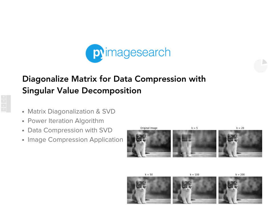
Finally, we choose different values of k for compression levels and plot the original and compressed images using matplotlib (Lines 28-45). The original image is displayed alongside the compressed images for various k values, illustrating how increasing k improves image quality while reducing the amount of data. By adjusting k, we can visually compare the effects of different levels of compression (Figure 7).

**Figure 7:** Illustration of how increasing $k$ improves the image quality of the reconstructed image (source: image by the author).

Summary

In this blog post, we explore the concept of matrix diagonalization and its applications in data compression using Singular Value Decomposition (SVD). We start by defining matrix diagonalization and explain its mathematical foundation. We then delve into SVD, a technique that decomposes a matrix into three simpler matrices: $U$ , $\Sigma$ , and $V^T$ . This decomposition helps in understanding the intrinsic properties of the matrix and paves the way for efficient data compression.

We further break down the process of diagonalizing a matrix with SVD using the Power Iteration algorithm. The step-by-step guide includes starting with a random vector, iteratively refining this vector, constructing singular vectors, deflating the matrix, and finally forming the matrices $U$ , $\Sigma$ , and $V^T$ . Each step is explained in a detailed yet simple manner to ensure comprehension. Additionally, we provide a method for calculating SVD using the Power Iteration algorithm, highlighting its practicality and effectiveness.

Finally, we discuss the application of SVD in data compression. By utilizing diagonalizable matrices, we can significantly reduce the size of data while maintaining its essential features. We illustrate this through an example of image data compression, where we implement SVD using NumPy and Pillow. By demonstrating how SVD can be applied to compress image data, we showcase its utility in real-world scenarios, making this technique accessible for various data compression tasks.

Citation Information

Mangla, P. “Diagonalize Matrix for Data Compression with Singular Value Decomposition,” PyImageSearch, P. Chugh, S. Huot, and P. Thakur, eds., 2025, https://pyimg.co/l1u02

@incollection{Mangla_2025_diagonalize-matrix-data-compression-singular-value-decomposition,
  author = {Puneet Mangla},
  title = {{Diagonalize Matrix for Data Compression with Singular Value Decomposition}},
  booktitle = {PyImageSearch},
  editor = {Puneet Chugh and Susan Huot and Piyush Thakur},
  year = {2025},
  url = {https://pyimg.co/l1u02},
}

To download the source code to this post (and be notified when future tutorials are published here on PyImageSearch), simply enter your email address in the form below!

Download the Source Code and FREE 17-page Resource Guide

Enter your email address below to get a .zip of the code and a FREE 17-page Resource Guide on Computer Vision, OpenCV, and Deep Learning. Inside you'll find my hand-picked tutorials, books, courses, and libraries to help you master CV and DL!