Hessian Matrix, Taylor Series, and the Newton-Raphson Method

Home » Blog » Hessian Matrix, Taylor Series, and the Newton-Raphson Method

Table of Contents

Hessian Matrix, Taylor Series, and the Newton-Raphson Method
Higher-Order Derivatives: The Hessian Matrix

Higher-Order Gradients
The Hessian Matrix

Taylor Series

Linearization
Taylor Series Expansion

Newton-Raphson Method
Summary

Citation Information

Hessian Matrix, Taylor Series, and the Newton-Raphson Method

In our previous lesson, we delved into the essentials of vector calculus by exploring partial derivatives and the Jacobian matrix, and their pivotal roles in optimization techniques such as Stochastic Gradient Descent (SGD). As we continue our journey through Vector Calculus, we turn our attention to more advanced concepts that further enhance our understanding of optimization algorithms and their applications in machine learning.

In this second lesson, we will dive deep into the Hessian matrix, the Taylor series, and the Newton-Raphson method. These mathematical tools are critical for analyzing and optimizing functions, particularly in multi-dimensional spaces. The Hessian matrix provides us with insights into the curvature of a function, while the Taylor series offers a way to approximate functions with polynomials. Together, these concepts set the stage for the Newton-Raphson method, a powerful iterative technique for optimizing objectives having frequent local optimums.

By understanding and applying these advanced topics, we aim to provide a solid foundation for tackling complex optimization problems. This lesson will equip us with the knowledge needed to fine-tune machine learning models more effectively, ensuring they perform at their best. So, let’s continue our exploration of vector calculus and uncover the mathematical principles that drive successful optimization strategies.

This lesson is the last of a 2-part series on Vector Calculus:

Partial Derivatives and Jacobian Matrix in Stochastic Gradient Descent
Hessian Matrix, Taylor Series, and the Newton-Raphson Method (this tutorial)

To learn how to implement the Newton-Raphson Method by using advanced concepts of vector calculus, just keep reading.

Higher-Order Derivatives: The Hessian Matrix

Higher-Order Gradients

Gradients and derivatives are also known as first-order derivatives. Higher-order derivatives or gradients means derivatives of derivatives.

Given a multivariate function $f(x_1, x_2, \dotsc, x_m): \mathbb{R}^m \rightarrow \mathbb{R}$ , higher-order gradients or derivatives are represented as follows:

$\displaystyle\frac{\partial^2 f}{\partial x_i^2}$ : second partial derivative of $f$ with respect to $x_i$ . In other words, the second-order derivative is the derivative of the first-order derivative $\displaystyle\frac{\partial}{\partial x_i} \displaystyle\frac{\partial f}{\partial x_i}$ .
$\displaystyle\frac{\partial^n f}{\partial x_i^n}$ is the $n^\text{th}$ order derivative of $f$ with respect to $x_i$ .
$\displaystyle\frac{\partial^2 f}{\partial x_j \partial x_i} = \displaystyle\frac{\partial}{\partial x_j} \displaystyle\frac{\partial f}{\partial x_i}$ : partial derivative obtained by first partial differentiating with respect to $x_i$ and then with respect to $x_j$ .
Similarly, $\displaystyle\frac{\partial^2 f}{\partial x_i \partial x_j} = \displaystyle\frac{\partial}{\partial x_i} \displaystyle\frac{\partial f}{\partial x_j}$ is the partial derivative obtained by first partial differentiating with respect to $x_j$ and then with respect to $x_i$ .

The Hessian Matrix

The Hessian matrix $H$ is a generalization of second-order derivatives for a multivariate function. It is a collection of all the second-order partial derivatives with the $(i,j)^\text{th}$ entry given as $H_{ij} = \displaystyle\frac{\partial^2 f}{\partial x_i \partial x_j}$ .

In other words,

$H = \begin{bmatrix} \displaystyle\frac{\partial^2 f}{\partial x_1^2} & . & . &. & \displaystyle\frac{\partial^2 f}{\partial x_1 \partial x_m} \\ . & .& . &. &. \\ . & .& \displaystyle\frac{\partial^2 f}{\partial x_i^2} &. &. \\ . & .& . &. &. \\ \displaystyle\frac{\partial^2 f}{\partial x_m \partial x_1} & . & . &. & \displaystyle\frac{\partial^2 f}{\partial x_m^2} \end{bmatrix} \in \mathbb{R}^{m \times m}$

Note that the partial derivatives $\displaystyle\frac{\partial^2 f}{\partial x_i \partial x_j} = \displaystyle\frac{\partial^2 f}{\partial x_j \partial x_i}$ because the variables $x_i$ and $x_j$ are independent of each other. The Hessian $H$ is, therefore, a symmetric matrix.

The following code snippet computes the Hessian matrix of a multivariate function $f(x_1, x_2, x_3) = x_1^2x_2^3x_3^4$ using the concept of second-order partial derivatives:

If you don’t have SciPy installed in your system, you can do so via pip install scipy.

import numpy as np
from scipy.misc import derivative
warnings.filterwarnings("ignore")

# objective function
def objective(x):
 return np.power(x[0], 2)*np.power(x[1], 3)*np.power(x[2], 4)

x0 = [-3, -2, 1] # m-dimensional input vector point to compute the Hessian at
fx0 = objective(x0) # objective evaluation

print("Value of f(x) at x0 = {} is {}".format(x0, fx0))

In this code, we begin by importing necessary libraries and suppressing warnings (Lines 1-3). We define an objective function (Lines 6 and 7) that takes a vector x as input and computes the value of the function $f(x) = x_0^2 \cdot x_1^3 \cdot x_2^4$ . We initialize x0 as the point at which we want to compute the Hessian matrix (Line 9) and evaluate the objective function at this point (Line 10), printing the result (Line 12).

hessian = [] # m x m matrix
for i in range(len(x0)):
    row_i = [] # second-order partial derivatives of the i-th row
    for j in range(len(x0)):
        # compute the i-j entry of the Hessian using second-order partial derivatives
        # first partial differentiating with respect to x_j
        pd_j = lambda x: derivative(lambda x_j: objective(x[:j] + [x_j] + x[j+1:]), x[j], dx=1e-6)
        # second partial differentiating with respect to x_i
        pd_ij = derivative(lambda x_i: pd_j(x0[:i] + [x_i] + x0[i+1:]), x0[i], dx=1e-6)

        print("Partial derivative w.r.t to first x_{} and then x_{} is : {}".format(j+1, i+1, np.round_(pd_ij, 2)))
        row_i.append(pd_ij)
    hessian.append(row_i)

print("Hessian of f(x) at x0 = {} is \n {}".format(x0, np.round_(hessian, 2)))

Next, we initialize an empty list hessian to store the second-order partial derivatives (Line 14). We loop through each element in x0 to compute the entries of the Hessian matrix (Line 15). For each element, we compute the first partial derivative with respect to x_j (Line 20), then compute the second partial derivative with respect to x_i (Line 22). We append these second-order partial derivatives to the corresponding row of the Hessian matrix (Line 25). Finally, we print the computed Hessian matrix, rounded to two decimal places (Line 28).

Output:

Value of f(x) at x0 = [-3, -2, 1] is -72
Partial derivative w.r.t to first x_1 and then x_1 is : -16.0
Partial derivative w.r.t to first x_2 and then x_1 is : -72.0
Partial derivative w.r.t to first x_3 and then x_1 is : 192.0
Partial derivative w.r.t to first x_1 and then x_2 is : -72.0
Partial derivative w.r.t to first x_2 and then x_2 is : -108.01
Partial derivative w.r.t to first x_3 and then x_2 is : 432.0
Partial derivative w.r.t to first x_1 and then x_3 is : 192.0
Partial derivative w.r.t to first x_2 and then x_3 is : 432.0
Partial derivative w.r.t to first x_3 and then x_3 is : -863.99
Hessian of f(x) at x0 = [-3, -2, 1] is 
 [[ -16.    -72.    192.  ]
 [ -72.   -108.01  432.  ]
 [ 192.    432.   -863.99]]

Taylor Series

Linearization

Recall that the derivative $df/dx$ of a function $f(x)$ at a point $x_0$ is given as follows:

$\displaystyle\frac{df(x_0)}{dx} = \lim_{\epsilon \rightarrow 0} \displaystyle\frac{f(x_0+\epsilon) - f(x_0)}{\epsilon}$ .

In assuming $x = x_0+h$ , the equation above can be rearranged and written as follows:

$f(x) = f(x_0) + \displaystyle\frac{df(x_0)}{dx} (x-x_0)$

where $\vert x - x_0 \vert < \epsilon$ and where $\epsilon \rightarrow 0$ . As can be seen, the derivatives $df/dx$ can now be used to approximate any function by a straight line around the point $x$ .

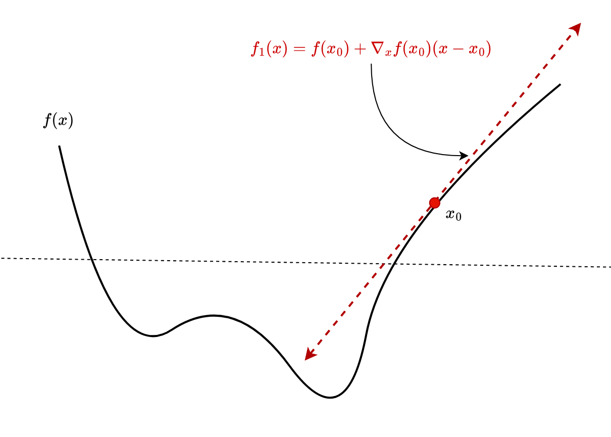
For multivariate, the linearization (Figure 1) above can be generalized as follows:

$f_1(x) = f(x_0) + \nabla_xf(x_0) (x - x_0)$

where $\nabla_x f(x_0)$ is the function gradient at the point $x_0$ . This approximation is locally accurate, but as we move farther from the point $x_0$ , it keeps getting worse.

**Figure 1:** Linear approximation of a polynomial with the Taylor series (source: image by the author).

Taylor Series Expansion

The linear approximation discussed above is a special case of the Taylor series through which we can approximate any function by an $n$ -degree polynomial (around the point $x_0$ ).

For a function, $f: \mathbb{R}^n \rightarrow \mathbb{R}$ , its Taylor expansion around the point $x_0$ can be written as follows:

$f(x) = \displaystyle\sum_{k=0}^{\infty} \displaystyle\frac{D^k_x f(x_0)}{k!} (x-x_0)^k$

where $D^k_x f(x_0)$ is the $k^\text{th}$ order derivative of the function $f$ with respect to $x$ , evaluated at the point $x_0$ .

To approximate the function $f$ with an $n$ -degree polynomial, we need to take the first $n+1$ terms of the Taylor series expansion.

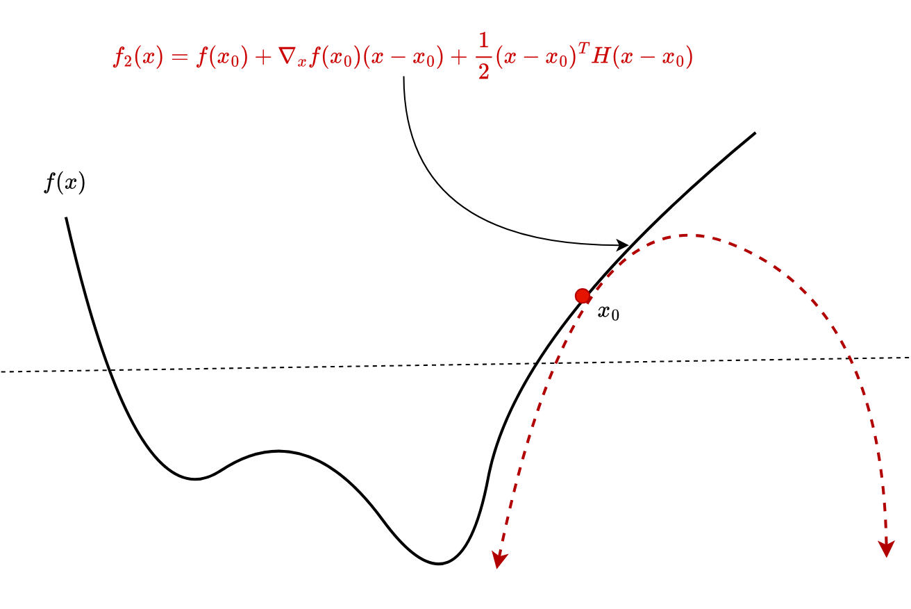
For example, the following polynomial approximates the function using a 2-degree polynomial around the point $x_0$ (Figure 2) :

$f_2(x) = f(x_0) + \nabla_xf(x_0)(x - x_0) + \displaystyle\frac{1}{2}(x - x_0)^T H(x_0) (x - x_0)$

where $H(x_0)$ is the Hessian of the function at the point $x_0$ , and $(.)^T$ is the matrix or vector transpose function.

**Figure 2:** Quadratic (2-degree) approximation of a polynomial with the Taylor series (source: image by the author).

Let’s consider the function $f(x) = f(x_1, x_2) = e^{x_1} + \sin(x_2)$ , which we seek to approximate by 1- and 2-degree polynomials around the point $x_0 = (1,1)$ . The gradient and Hessian of the function are given as follows:

$\nabla_x f(x) = [ e^{x_1}, \cos(x_2) ]$

$H(x) = \begin{bmatrix} e^{x_1} & 0 \\ 0 & -\sin(x_2) \end{bmatrix}$

Using the Taylor series expansion, the 1-degree polynomial (or linear) approximation $f_1(x)$ can be written as follows:

$f_1(x) = f(x_0) + \nabla_xf(x)(x - x_0) = e + \sin(1) + e(x_1-1) + \cos(1)(x_2 -1)$

Similarly, the 2-degree polynomial approximation $f_2(x)$ can be written as follows:

$f_2(x) = e + \sin(1) + e(x_1-1) + \cos(1)(x_2 -1) + \displaystyle\frac{1}{2}e(x_1-1)^2 -\frac{1}{2}\sin(1)(x_2 -1)^2$

The code snippet below implements and validates the approximations above:

import numpy as np
from scipy.misc import derivative
import matplotlib.pyplot as plt
warnings.filterwarnings("ignore")

# objective function
def objective(x):
 return np.round(np.exp(x[0]) + np.sin(x[1]), 2)

# one-degree polynomial approximation or linearization
def linear_approximation(x, x0):
    return np.round(objective(x0) +  \
                    np.exp(x0[0])*(x[0] - x0[0]) + np.cos(x0[1])*(x[1] - x0[1]), 2)

# two-degree polynomial approximation
def quadratic_approximation(x, x0):
    return np.round(objective(x0) \
            + np.exp(x0[0])*(x[0] - x0[0]) + np.cos(x0[1])*(x[1] - x0[1]) \
            + 0.5*np.exp(x0[0])*(x[0] - x0[0])*(x[0] - x0[0]) \
            - 0.5*np.sin(x0[1])*(x[1] - x0[1])*(x[1] - x0[1]), 2)

In this code, we start by importing necessary libraries (Lines 29-31) and define an objective function (Lines 35 and 36) that takes a vector x and returns the rounded value of $e^{x[0]} + \sin(x[1])$ . We then define two functions for polynomial approximations: linear_approximation (Lines 39-41) and quadratic_approximation (Lines 44-48). These functions create linear and quadratic approximations of the objective function around a point x0 by using first and second derivatives, respectively.

x0 = [1, 1] # m-dimensional input vector point to compute the Hessian at
fx0 = objective(x0) # objective evaluation

xs = [[1.1, 0.9], [0.9, 1.1], [1.5, 0.5], [0.5, 1.5]] # points to evaluate

# print actual function value, its linear and quadratic approximation
for x in xs:
    print("Evaluating at x = {}".format(x))
    print("Actual f(x) : {} ".format(objective(x)))
    print("Linear approximation of f(x) : {}".format(linear_approximation(x, x0)))
    print("Quadratic approximation of f(x) : {}".format(quadratic_approximation(x, x0)))
    print("-----")

# plot all the curves for graphic visualization
plt.figure(figsize=(30,10))
plt.rcParams.update({'font.size': 30})
x1s, x2s = np.arange(x0[0] - 0.75, x0[0] + 0.75, 0.05), np.arange(x0[1] - 0.75, x0[1] + 0.75, 0.05)

fs = {
    0: ["Actual f(x)", objective],
    1: ["Linear approx. of f(x)", lambda x: linear_approximation(x, x0)],
    2: ["Quadratic approx. of f(x)", lambda x: quadratic_approximation(x, x0)]
}
for i in range(3):
    plt.subplot(1, 3, i+1)
    zs = [[fs[i][1]([x1,x2]) for x2 in x2s] for x1 in x1s]
    plt.contourf(x1s, x2s, zs)

    plt.title(fs[i][0])
    plt.xlabel('x1')
    plt.ylabel('x2')

    plt.scatter(x0[0], x0[1], color='yellow', linewidths=6, label='(x1, x2)')
    plt.legend()

plt.show()

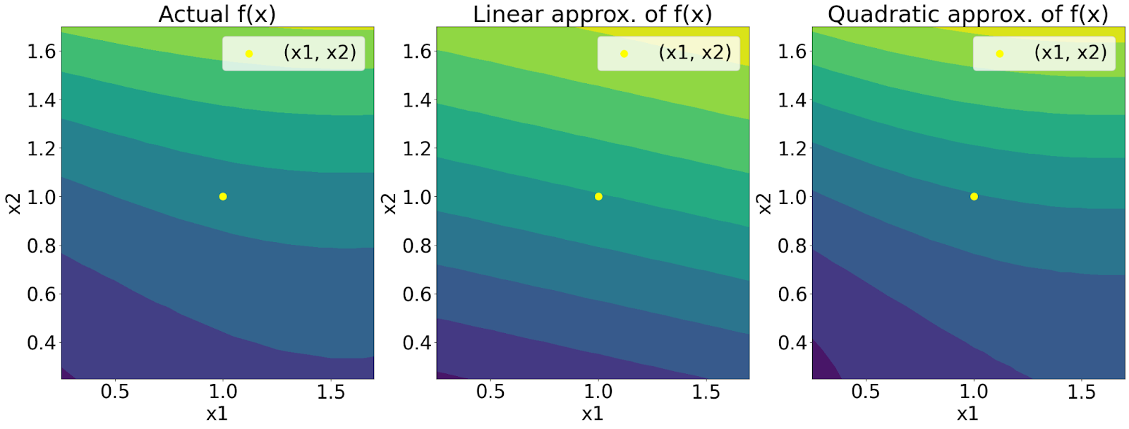
Next, we initialize x0 as the point of interest (Line 50) and evaluate the objective function at this point (Line 51). We define a list of points xs to evaluate the function and its approximations (Line 53). For each point in xs, we print the actual function value, its linear, and quadratic approximations (Lines 56-61). Finally, we plot these values for visualization (Lines 64-85). The plots show the actual function, linear approximation, and quadratic approximation, with x0 highlighted on each plot (Figure 3). This helps us visually compare the approximations to the actual function.

Output:

Evaluating at x = [1.1, 0.9]
Actual f(x) : 3.79 
Linear approximation of f(x) : 3.78
Quadratic approximation of f(x) : 3.79
-----
Evaluating at x = [0.9, 1.1]
Actual f(x) : 3.35 
Linear approximation of f(x) : 3.34
Quadratic approximation of f(x) : 3.35
-----
Evaluating at x = [1.5, 0.5]
Actual f(x) : 4.96 
Linear approximation of f(x) : 4.65
Quadratic approximation of f(x) : 4.88
-----
Evaluating at x = [0.5, 1.5]
Actual f(x) : 2.65 
Linear approximation of f(x) : 2.47
Quadratic approximation of f(x) : 2.71
-----

**Figure 3:** Linear (1-degree) vs. Quadratic (2-degree) approximation of a polynomial with the Taylor series (source: image by the author).

Newton-Raphson Method

Newton’s methods are a class of optimization algorithms that leverage second-order information (e.g., Hessians) to achieve faster and more efficient convergence. In contrast, the gradient descent algorithms, like the Stochastic Gradient Descent (as discussed in the previous lesson), depend solely on first-order gradient information.

The idea of Newton’s method is to utilize the curvature information present in Hessians to obtain a more accurate approximation of the function near the optimum.

Recall the 2-degree Taylor series expansion of our objective $f(x)$ around a point $x_t$ (at the time $t$ ) as follows:

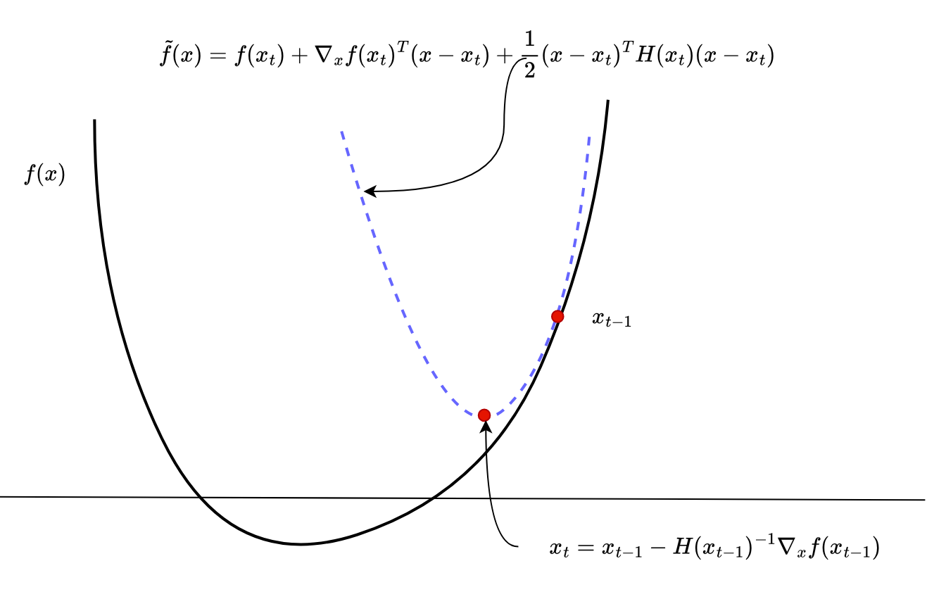
$\tilde{f}(x) = f(x_t) + \nabla_x f(x_t)^T(x-x_t) + \displaystyle\frac{1}{2}(x-x_t) ^T H(x_t) (x-x_t)$

where $\nabla_x f(x_t)$ and $H(x_t)$ represents the gradient and the Hessian of the function $f(x)$ at $x = x_t$ , respectively.

Because the function $\tilde{f}(x)$ locally approximates $f(x)$ around $x_t$ , the minimum value of $\tilde{f}(x)$ will provide us the minimum value of the original function $f(x)$ around $x_t$ .

Because $\tilde{f}(x)$ is a quadratic (convex) function, we can find its minimum by setting its gradient with respect to $x$ as 0, as given below:

$\nabla_x \tilde{f}(x) = \nabla_x f(x_t) + H(x_t)(x-x_t) = 0$

Solving the equation above gives us the updated rule of the Newton algorithm at time $t+1$ as follows:

$x_{t+1} = x_t - H(x_t)^{-1} \nabla_x f(x_t)$

The method uses this equation to iteratively update the guess $x_t$ until it converges to the optimal solution of the function. The algorithm is said to converge once the guess stops changing.

$\Vert \ x_{t+1} - x_t \ \Vert_2 < \epsilon$

Figure 4 illustrates how Newton’s method works:

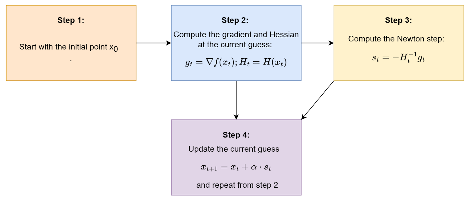
**Figure 4:** Illustration of the Newton-Raphson method (source: image by the author).

Here’s a step-by-step explanation of how it works (Figure 5):

Initial guess: Start with an initial guess $x_0$ .
Gradient and Hessian: Calculate the gradient (first derivative) and the Hessian (second derivative) of the function at the current guess $x_t$ .
Newton step: Compute the Newton step, which is the direction in which the function decreases the fastest. This is given by the negative inverse of the Hessian times the gradient (i.e., $-H(x_t)^{-1} \nabla_x f(x_t)$ ).
Update: Update the current guess by taking a step in the direction of the Newton step with the step size $\alpha$ (i.e., $x_{t+1} = x_t - \alpha \cdot H(x_t)^{-1} \nabla_x f(x_t)$ ).
Iteration: Repeat Steps 2-4 until the change in function value or change in $x$ is below a certain threshold.

**Figure 5:** Block diagram illustrating the steps in the Newton-Raphson method (source: image by the author).

In Figure 4, the black line represents the objective function, and the dotted blue line represents the 2-degree polynomial approximation of the objective function at the current point, $x_{t-1}$ .

Newton’s method utilizes the curvature information present in Hessians to approximate the function by a quadratic polynomial at the current point $x_{t-1}$ . It then updates the current point with the optimum of that approximated function $x_t$ .

The code below implements the Newton-Raphson method algorithm on the Rosenbrock function $f(x, y) = (1-x)^2 + 100(y-x^2)^2$ , which is a non-convex function with a global optimum at $f(1,1) = 0$ and several local optimums around it. These local optimums prevent the standard gradient descent algorithms (e.g., stochastic gradient descent) from converging to the global optimal solution.

import numpy as np
import matplotlib.pyplot as plt

# define the Rosenbrock function
def objective(x,y):
     return (1 - x)**2 + 100 * (y - x**2)**2

# gradient of objective
def gradient(x, y):
     dx = -2 * (1 - x) - 400 * x * (y - x**2)
     dy = 200 * (y - x**2)
     return np.array([dx, dy])

def hessian(x, y):
     dxx = 2 -400*y + 1200*(x**2)
     dyy = 200
     dxy = -400*x

     return np.array([[dxx, dxy], [dxy, dyy]])

In this code, we start by defining the Rosenbrock function as our objective function (Lines 90 and 91). This is a common test problem for optimization algorithms, known for its banana-shaped valley. We also define functions to compute the gradient (Lines 94-97) and Hessian matrix (Lines 99-104) of the objective function.

T = 5 # total iterations
x_t, y_t = 3, -2 # initial point
path = [[x_t, y_t]]
alpha = 1

for t in range(T):
     grad = gradient(x_t, y_t) # compute gradient
     H = hessian(x_t, y_t) # compute gradient
     Hinv = np.linalg.inv(H)

     newton_step = -np.dot(Hinv, grad)

     x_t = x_t + alpha*newton_step[0]
     y_t = y_t + alpha*newton_step[1]

     if t%1 == 0 or t  == T-1:
          path.append([x_t, y_t])
          print("(x,y) at step {} = ({:.3f}, {:.3f})".format(t, x_t, y_t))

We initialize the total number of iterations T, the starting point (x_t, y_t), and set the learning rate alpha (Lines 106-109). We then enter a loop to perform the Newton-Raphson method for optimization. Within each iteration, we compute the gradient and Hessian matrix, calculate the Newton step, update the variables, and store the path for visualization (Lines 111-123).

print("Optimal solution (x,y)  = ({:.3f}, {:.3f})".format(x_t, y_t))
print("Optimal objective f(x,y)  = {:.3f}".format(objective(x_t, y_t)))

# plot the curve for graphic visualization
plt.figure(figsize=(5,5))
plt.rcParams.update({'font.size': 11})

xs, ys = np.arange(-10.0, 10.0, 0.05), np.arange(-10.0, 10.0, 0.05)
zs = [[objective(x, y) for x in xs] for y in ys]
plt.contourf(xs, ys, zs) # Visualize the contour plot

plt.title('Filled Contour Plot')
plt.xlabel('y')
plt.ylabel('x')

# visualize the optimal point
plt.scatter(y_t, x_t, linewidth=6, color='orange', label='optimum, Loss = {:.2f}'.format(objective(x_t, y_t)))

for i in range(len(path) -1):
     plt.arrow(path[i][1], path[i][0], (path[i+1][1] -path[i][1]), (path[i+1][0] - path[i][0]), color='yellow', width=0.02)

plt.show()

After completing the optimization, we print the optimal solution and its objective function value (Lines 125 and 126). For visualization, we create a contour plot of the objective function using plt.contourf, highlight the optimal point, and display the path of iterations with arrows (Lines 129-144). Finally, we display the plot with plt.show (Line 146), which visually illustrates the optimization process and the path taken to reach the optimal solution (Figure 6).

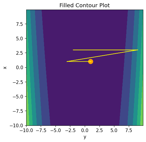
**Figure 6:** Finding global minima of the Rosenbrock function using the Newton-Raphson method (source: image by the author).

Output:

(x,y) at step 0 = (2.999, 8.995)
(x,y) at step 1 = (1.000, -2.994)
(x,y) at step 2 = (1.000, 1.001)
(x,y) at step 3 = (1.000, 1.000)
(x,y) at step 4 = (1.000, 1.000)
Optimal solution (x,y)  = (1.000, 1.000)
Optimal objective f(x,y)  = 0.000

Summary

In this blog post, we delve into the fascinating interplay between the Hessian matrix, the Taylor series, and the Newton-Raphson method. We begin by exploring higher-order derivatives, focusing on the Hessian Matrix and its significance in optimization. Next, we discuss higher-order gradients and their applications.

We then introduce the Taylor series, starting with linearization and progressing to the Taylor series expansion, demonstrating how these mathematical tools provide approximations of functions. Finally, we examine the Newton-Raphson method, a powerful technique for finding roots of functions.

Throughout the post, we connect these concepts, highlighting their roles in optimization and computational mathematics. By the end, we offer a comprehensive understanding of these fundamental tools and their applications.

Citation Information

Mangla, P. “Hessian Matrix, Taylor Series, and the Newton-Raphson Method,” PyImageSearch, P. Chugh, S. Huot, and P. Thakur, eds., 2025, https://pyimg.co/1pqgw

@incollection{Mangla_2025_partial-derivatives--jacobian-matrix-sgd,
  author = {Puneet Mangla},
  title = {{Hessian Matrix, Taylor Series, and the Newton-Raphson Method}},
  booktitle = {PyImageSearch},
  editor = {Puneet Chugh and Susan Huot and Piyush Thakur},
  year = {2025},
  url = {https://pyimg.co/1pqgw},
}

To download the source code to this post (and be notified when future tutorials are published here on PyImageSearch), simply enter your email address in the form below!

Download the Source Code and FREE 17-page Resource Guide

Enter your email address below to get a .zip of the code and a FREE 17-page Resource Guide on Computer Vision, OpenCV, and Deep Learning. Inside you'll find my hand-picked tutorials, books, courses, and libraries to help you master CV and DL!

Hessian Matrix, Taylor Series, and the Newton-Raphson Method

Higher-Order Derivatives: The Hessian Matrix

Higher-Order Gradients

The Hessian Matrix

Taylor Series

Linearization

Taylor Series Expansion

Newton-Raphson Method

Summary

Citation Information

Download the Source Code and FREE 17-page Resource Guide

About the Author

Comment section

PyImageSearch University

ImageNet: VGGNet, ResNet, Inception, and Xception with Keras

Install OpenCV 4 on Raspberry Pi 4 and Raspbian Buster

Building a Dataset for Triplet Loss with Keras and TensorFlow

Topics

Books & Courses

PyImageSearch

Download the Source Code and FREE 17-page Resource Guide

About the Author

Partial Derivatives and Jacobian Matrix in Stochastic Gradient Descent

Hessian Matrix, Taylor Series, and the Newton-Raphson Method

Comment section

Similar articles

You can learn Computer Vision, Deep Learning, and OpenCV.

Footer

Topics

Books & Courses

PyImageSearch

Access the code to this tutorial and all other 500+ tutorials on PyImageSearch

What's included in PyImageSearch University?