Scaling Kaggle Competitions Using XGBoost: Part 3

---

Table of Contents

---

Scaling Kaggle Competitions Using XGBoost: Part 3

We continue our journey into understanding XGBoost, but there is one penultimate stop we need to make before deep diving into the nitty gritty of Extreme Gradient Boosting. We are not quite at the stage of embracing the “Extreme” nature of Gradient Boosting yet, as we are yet to demystify Gradient Boosting itself.

In this blog post, we will thoroughly understand what Gradient Boosting is and understand the math behind this beautiful concept.

In this tutorial, you will learn about Gradient Boosting, the final precursor to XGBoost.

This lesson is the 3rd of a 4-part series on Deep Learning 108:

1. Scaling Kaggle Competitions Using XGBoost: Part 1
2. Scaling Kaggle Competitions Using XGBoost: Part 2
3. Scaling Kaggle Competitions Using XGBoost: Part 3 (this tutorial)
4. Scaling Kaggle Competitions Using XGBoost: Part 4

To learn how to utilize Gradient Boosting, just keep reading.

---

Scaling Kaggle Competitions Using XGBoost: Part 3

---

Gradient Boost at a Glance

In the first blog post of this series, we went through basic concepts like ensemble learning and decision trees. To refresh your memory, we recommend going through the first blog post of this series once again.

To recap: ensemble learners are normally a group of weak algorithms working together to produce quality output. Throughout this series, we have investigated algorithms by applying them to decision trees. So, it is important that you have a clear idea of how decision trees work.

The concept of Gradient Boosting works very similarly to how AdaBoost operates (see previous blog post). The errors generated by the past predictor tree are used as information by the next predictor tree to improve its result. However, the two algorithms are very different.

---

AdaBoost vs. Gradient Boosting

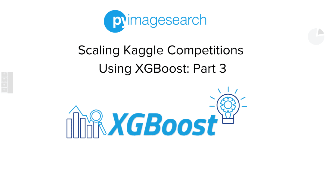
For a quick reminder on how AdaBoost works, take a look at Table 1.

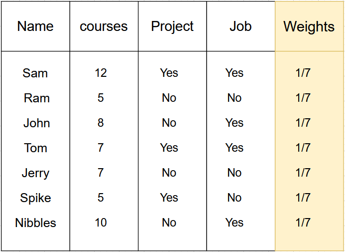
Each sample is given a weight. Once the initial decision stump is created based on the features, we have certain samples which will get wrongly classified in those particular stumps. The next step is to focus on correcting those wrongly classified samples and change the weights based on the samples that need more focus than others (Table 2).

Instead of working with sample weights, Gradient Boosting works with “residuals.” In the case of regression, residuals are nothing but the difference between the predicted values and the actual labels. These residuals tell us how far off our predictions are from the actual labels and become the labels themselves for subsequent tree creations (we will work these out in detail in the next section).

In short, AdaBoost works with sample weights focusing on wrongly classified samples to make sure they are corrected in subsequent stumps. But the Gradient Boosting algorithm is created so that samples get individual focus without additional weights to affect preferences. Also, the significance of stumps in the final say of the output is a key point in AdaBoost, which is not present in Gradient Boosting.

If the terms thrown around for Gradient Boosting in this section has you “stumped,” don’t worry; a detailed analysis is in order.

---

Gradient Boosting Dissected

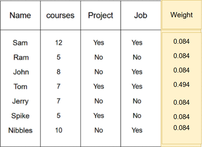
Consistent with our previous posts, we will consider a dummy dataset to better understand the concepts (Table 3).

Note that this first example will focus on Gradient Boosting for regression. Gradient Boosting for classification is slightly different but is based on the same foundational principles you’ll learn for the regression task.

So we start with a dummy dataset with 4 samples. The Courses and Credit columns are the features, while the Score column is the label. The mathematical way of expressing this is , where and are nothing but features and labels of the th sample, respectively.

If you check the Wikipedia page for Gradient Boosting, there’s a section dedicated to the math equations used in Gradient Boosting (Figure 1).

Now at a glance, this might seem super complicated but don’t worry, stick with us, and we will systematically break this down for you.

Since we already have spoken about the training set, the next thing to note here is the differentiable loss function . This is where is simply the predictions, and is the corresponding labels, with the algorithm being run for (a choice dependent on the user) iterations.

Step 1 is to initialize a model (in our case, a tree with a singular node). Now the equation might feel confusing to you at first glance, but it really isn’t. simply means that we need to solve for a prediction (The prediction) such that it minimizes the equation.

Before we jump into that, let’s talk about the loss function. The standard go-to here is the squared loss with a constant of before it. So it comes to . Note that these functions have constants like this since the loss functions require to be differentiated for backpropagation, and the differentiated loss function will look like: .

To find the ideal value for for our dummy dataset, we will:

• 
• 
• 

which gives us the value for .

This becomes our first predictor, the average of all the labels.

Step 2 runs for the number of iterations you set it to but don’t get scared at how the equation looks. Under Step 2, we first calculate the “pseudo-residuals.” Now, as we have established that the loss function differentiated simply gives us (Table 4).

This gives us our first tables and residuals with which to work. To make things easier, you can consider this averaged-out node as your baseline regressor. The second part of the step involves us creating another decision tree, but this time it would be to predict the residuals. Let’s see what it turns out to be (Figure 2).

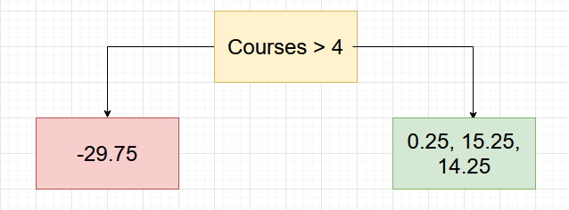
For ease of explanation, we will be using this simple tree. In practical cases, you will have much better trees. The problem with this tree is that one of the nodes has multiple labels, which can’t be a possibility.

Hence, we need to figure out a single output that represents the node. We can use the equation we have used in Step 1 just for the green node and solve for , which would give us the representative value as .

Now, for any new sample with courses greater than , the green node will be represented by a single value, .

But now the question remains: how will we make use of this? For this, we move to the final part of Step 2.

• Till now, we have our baseline predictor (the average of labels).
• Since the average will not predict correctly for most samples, we calculate the residuals. Note that if you add the residuals to our initial prediction, we get the perfect labels for each training sample. Unfortunately, that means we are severely overfitting on the training data. For this reason, we compute a “learning rate” for each subsequent tree to take small steps toward our eventual result.
• We create a decision tree to predict the residuals and ensure each leaf node has a single output representation.
• Now, our updated model becomes .

Let’s see what happens in the case of our dummy data (Table 5):

So for the case of the data entry “Tom,” if we try to predict using our created trees, we get:

• from our baseline classifier
• from the second tree

Adding these two values, we get as our prediction. Notice that it is still less than the actual label , but better than our initial baseline prediction. Hence, with our first tree, we have indeed made progress toward the actual labels. We keep repeating this process and calculating residuals to slowly inch closer to the actual labels.

This concludes the working of gradient boosting using regression. Next, we will use Gradient Boosting on an actual dataset and analyze the results.

---

Configuring Your Development Environment

To follow this guide, you need to have the OpenCV library installed on your system.

Luckily, OpenCV is pip-installable:

$ pip install opencv-contrib-python

If you need help configuring your development environment for OpenCV, we highly recommend that you read our pip install OpenCV guide — it will have you up and running in a matter of minutes.

---

Having Problems Configuring Your Development Environment?

All that said, are you:

• Short on time?
• Learning on your employer’s administratively locked system?
• Wanting to skip the hassle of fighting with the command line, package managers, and virtual environments?
• Ready to run the code right now on your Windows, macOS, or Linux system?

Then join PyImageSearch University today!

Gain access to Jupyter Notebooks for this tutorial and other PyImageSearch guides that are pre-configured to run on Google Colab’s ecosystem right in your web browser! No installation required.

And best of all, these Jupyter Notebooks will run on Windows, macOS, and Linux!

---

Setting Up Our Project

Like XGBoost, it is easy to plug in the Gradient Boost algorithm using the sci-kit library.

# import necessary packages
import pandas as pd
import xgboost as xgb
from sklearn.datasets import load_iris
from sklearn.model_selection import train_test_split
from sklearn.metrics import mean_squared_error 
from sklearn import ensemble

On Lines 2-7, we import the necessary packages, including the Iris dataset, XGBoost, and sci-kit ensemble package.

# load the iris dataset and create the dataframe
iris = load_iris()
X = pd.DataFrame(iris.data, columns=iris.feature_names)
y = pd.Series(iris.target) 
 
# split the dataset 
xTrain, xTest, yTrain, yTest = train_test_split(X, y)

Next, we do the preliminary data setup. On Line 10, we loaded the iris dataset and stored it inside a dataframe (Lines 10 and 11).

We split the dataset into training and test splits (Line 15).

Next, we will compare the scores of XGBoost and Gradient Boosting.

---

Comparing XGboost and Gradient Boost Results

We will initialize the two algorithms with similar parameters to make the testing conditions as equal as possible.

# initialize the gradient boosting algorithm
gradientBooster = ensemble.GradientBoostingRegressor(n_estimators = 50,
    max_depth =  8,
    learning_rate = 1,
    criterion = 'squared_error'
)

On Lines 18-22, we have initialized the Gradient Boost algorithm with 50 trees, a maximum tree depth of 8, a learning rate of 1, and a simple squared error as our loss function.

# fit the training data 
gradientBooster.fit(xTrain, yTrain)
 
# check the score of the algorithm on test data
gradientBooster.score(xTest, yTest)

Next, we simply fit the training data and score the trained algorithm on the test set (Lines 25-28). We shall analyze the scores later.

# define the XGBoost regressor according to your specifications
xgbModel = xgb.XGBRegressor(
    n_estimators=50,
    reg_lambda=2,
    gamma=0,
    max_depth=8
)

The XGBoost regressor object is initialized on Lines 31-36, with 50 trees, a regularization value of 2, and a max tree depth of 8. There are several other parameters we can tweak, but for now, we are choosing to keep it simple.

# fit the training data in the model
xgbModel.fit(xTrain, yTrain)
 
# check the score of the algorithm on test data
xgbModel.score(xTest, yTest)

As we had done for the Gradient Boost object, we fit the training data on the algorithm and scored it on the test set (Lines 39-42).

The Gradient Boost algorithm obtained a testing accuracy of 96.4, while the XGBoost algorithm obtained a 97.09.

---

---

Summary

Although XGBoost had better accuracy, Gradient Boost came really close to beating it. As XGBoost is built on Gradient Boost principles, it is important to understand how it works. The simple idea is to utilize ensemble learnings and pseudo-linear residuals to improve the prediction each time.

The nature of this algorithm is such that each tree will, in most cases, improve upon the previous result, be it by a tiny step. With the concept of Gradient Boost under our grasp, we are finished with the precursors for XGBoost, which will be our final destination in the next part of this series.

---

Citation Information

Martinez, H. “Scaling Kaggle Competitions Using XGBoost: Part 3,” PyImageSearch, P. Chugh, A. R. Gosthipaty, S. Huot, K. Kidriavsteva, R. Raha, and A. Thanki, eds., 2023, https://pyimg.co/8he0y

@incollection{Martinez_2023_XGBoost3,
  author = {Hector Martinez},
  title = {Scaling {Kaggle} Competitions Using {XGBoost}: Part 3},
  booktitle = {PyImageSearch},
  editor = {Puneet Chugh and Aritra Roy Gosthipaty and Susan Huot and Kseniia Kidriavsteva and Ritwik Raha and Abhishek Thanki},
  year = {2023},
  note = {https://pyimg.co/8he0y},
}

---

---

To download the source code to this post (and be notified when future tutorials are published here on PyImageSearch), simply enter your email address in the form below!