Torch Hub Series #3: YOLOv5 and SSD — Models on Object Detection

In my childhood, the movie Spy Kids was one of my favorite things to watch on television. Seeing kids of my age using futuristic gadgets to save the world and win the day might have been a common trope, but it still was fun to watch. Amongst things like Jetpacks and self-driving cars, my favorite was smart sunglasses, which could identify objects and people around you (it also doubled as a binocular), something like Figure 1.

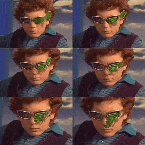
Understandably, the conception of these gadgets in real life was hard to fathom at that time. However, now that we are in 2022, a self-driving car company (Tesla) is at the top of the motor industry, and detecting objects from real-time videos is a piece of cake!

So today, apart from understanding a fever dream of a young me, we will see how PyTorch Hub makes exploring these domains as easy.

In this tutorial, we will learn the intuition behind models like YOLOv5 and SSD300 and harness their powers using Torch Hub.

This lesson is part 3 of a 6-part series on Torch Hub:

1. Torch Hub Series #1: Introduction to Torch Hub
2. Torch Hub Series #2: VGG and ResNet
3. Torch Hub Series #3: YOLOv5 and SSD — Models on Object Detection (this tutorial)
4. Torch Hub Series #4: PGAN — Model on GAN
5. Torch Hub Series #5: MiDaS — Model on Depth Estimation
6. Torch Hub Series #6: Image Segmentation

To learn how to utilize YOLOv5 and SSD300, just keep reading.

Torch Hub Series #3: YOLOv5 and SSD — Models on Object Detection

Object Detection at a Glance

Object Detection is undoubtedly a very alluring domain at first glance. Making a machine identify the exact position of an object inside an image makes me believe that we are another step closer to achieving the dream of mimicking the human brain. But even if we keep that aside, it has a variety of critical usage in today’s world. From Face Detection systems to helping Self-Driving Cars safely navigate, the list goes on. But how does it work exactly?

There are many methods to achieve Object Detection, using machine learning as the core idea. For example, in this blog post about training an object detector from scratch in PyTorch, we simply have an architecture that takes in the image as input and outputs 5 things; the class of the detected object and start and end values for the height and width of the object’s bounding box.

Essentially, we are grabbing annotated images and passing them through a simple CNN with an output of size 5. Consequently, like with every new thing developed in Machine Learning, more complex and intricate algorithms followed to improve it.

Note, if you think about the methodology I just mentioned in the previous paragraph, it might work just fine for images with a single object to detect. However, this will almost certainly hit a roadblock when multiple objects are inside a single image. So, to tackle this and other constraints like efficiency, we move on to YOLO(v1).

YOLO, or “You Only Look Once” (2015), introduced an ingenious way to tackle the shortcomings of a simple CNN detector. We split each image into an S×S grid, getting object positions corresponding to each cell. Of course, some cells won’t have any objects, while others will appear in multiple cells. Take a look at Figure 2.

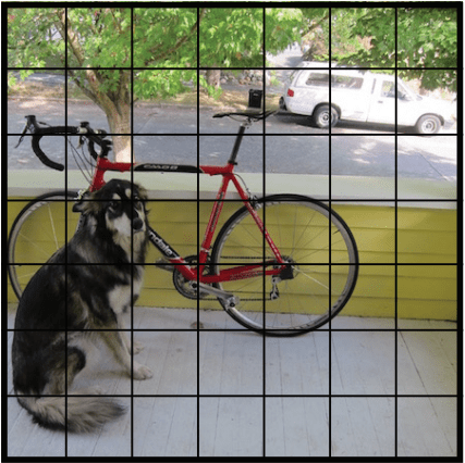
It’s important to know the objects’ midpoint, height, and width for the complete image. Each cell will then output a probability value (probability of an object being in the cell), the detected object class, and the bounding box values unique to the cell.

Even if each cell can detect only one object, the existence of multiple cells nullifies the constraint. The result can be seen in Figure 3.

Despite great results, YOLOv1 had a major flaw; the closeness of objects inside an image often made the model miss some objects. Since its inception, several successors have been published, like YOLOv2, YOLOv3, and YOLOv4, each being better and faster than its predecessor. This brings us to one of today’s spotlights, YOLOv5.

Glenn Jocher, the creator of YOLOv5, decided against writing a paper and instead open sourced the model through GitHub. Initially, that raised a lot of concern since people thought the results weren’t reproducible. However, that notion was swiftly broken, and today, YOLOv5 is one of the official state-of-the-art models hosted in the Torch Hub showcase.

To understand what improvements YOLOv5 brought, we have to go back to YOLOv2. Amongst other things, YOLOv2 introduced the concept of anchor boxes. A series of predetermined bounding boxes, anchor boxes are of specific dimensions. These boxes are chosen depending on object sizes in your training datasets to capture the scale and aspect ratio of various object classes you want to detect. The network predicts the probabilities corresponding to the anchor boxes rather than the bounding boxes themselves.

But in practice, hoisted YOLO models are most often trained on the COCO dataset. This led to a problem since the custom dataset might not have the same anchor box definitions. YOLOv5 tackles this problem by introducing auto-learning anchor boxes. It also utilizes mosaic augmentation, mixing random images to make your model adept at identifying objects at a smaller scale.

The second item from today’s spotlight is the SSD or Single Shot MultiBox Detector model for object detection. The SSD300 originally used a VGG backbone for adept feature detection and utilized Szegedy‘s work on MultiBox, a method for quick class-agnostic bounding box coordinate recommendations, inspired SSD’s bounding box regression algorithm. Figure 4 shows the SSD architecture.

Inspired by inception-net, the Multibox architecture created by Szegedy utilizes a multiscale convolutional architecture. Multibox uses a series of normal convolutional and 1×1 filters (changing channel size but keeping height and width intact) to incorporate a multiscale bounding box and confidence prediction model.

The SSD was famous for utilizing multiscale feature maps instead of single feature maps for detections. This allowed for finer detections and more granularity in the predictions. Using these feature maps, the anchor boxes for object predictions were generated.

It had outperformed its compatriots when it came out, especially in speed. Today we’ll be using Torch Hub’s showcased SSD, which uses a ResNet instead of a VGG net as its backbone. Also, some other changes, like removing some layers according to the Speed/accuracy trade-offs for modern convolutional object detectors paper, were applied to the model.

Today, we’ll learn how to harness the power of these models using Torch Hub and test them with our custom datasets!

Configuring Your Development Environment

To follow this guide, you need to have the OpenCV library installed on your system.

Luckily, OpenCV is pip-installable:

$ pip install opencv-contrib-python

If you need help configuring your development environment for OpenCV, we highly recommend that you read our pip install OpenCV guide — it will have you up and running in a matter of minutes.

Having Problems Configuring Your Development Environment?

All that said, are you:

• Short on time?
• Learning on your employer’s administratively locked system?
• Wanting to skip the hassle of fighting with the command line, package managers, and virtual environments?
• Ready to run the code right now on your Windows, macOS, or Linux system?

Then join PyImageSearch University today!

Gain access to Jupyter Notebooks for this tutorial and other PyImageSearch guides that are pre-configured to run on Google Colab’s ecosystem right in your web browser! No installation required.

And best of all, these Jupyter Notebooks will run on Windows, macOS, and Linux!

Project Structure

We first need to review our project directory structure.

Start by accessing the “Downloads” section of this tutorial to retrieve the source code and example images.

From there, take a look at the directory structure:

!tree . 
.
├── output
│   ├── ssd_output
│   │   └── ssd_output.png
│   └── yolo_output
│       └── yolo_output.png
├── pyimagesearch
│   ├── config.py
│   ├── data_utils.py
├── ssd_inference.py
└── yolov5_inference.py

First, we have the output directory, which will house the outputs we’ll get from each model.

In the pyimagesearch directory, we have two scripts:

• config.py: This script houses the end to end configuration pipeline of the project
• data_utils.py: This script contains some helper functions for data processing

In the main directory, we have two scripts:

• ssd_inference.py: This script contains the SSD model inference for custom images.
• yolov5_inference.py: This script contains the YOLOv5 model inference for custom images.

Downloading the Dataset

The first step is to configure our dataset according to our needs. Like in the previous tutorial, we’ll be using the Dogs & Cats Images dataset from Kaggle, owing to its relatively small size.

$ mkdir ~/.kaggle
$ cp <path to your kaggle.json> ~/.kaggle/
$ chmod 600 ~/.kaggle/kaggle.json
$ kaggle datasets download -d chetankv/dogs-cats-images
$ unzip -qq dogs-cats-images.zip
$ rm -rf "/content/dog vs cat"

To use the dataset, you’ll need to have your own unique kaggle.json file to connect to the Kaggle API (Line 2). The chmod 600 command on Line 3 gives the user full access to read and write files.

This is followed by the kaggle datasets download command (Line 4) allows you to download any dataset hosted on their website. Finally, unzip the file and delete the unnecessary additions (Lines 5 and 6).

Let’s move on to the configuration pipeline.

Configuring the Prerequisites

Inside the pyimagesearch directory, you’ll find a script called config.py. This script will house the complete end-to-end configuration pipeline of our project.

# import the necessary packages
import torch
import os

# define the root directory followed by the test dataset paths
BASE_PATH = "dataset"
TEST_PATH = os.path.join(BASE_PATH, "test_set")

# specify image size and batch size
IMAGE_SIZE = 300
PRED_BATCH_SIZE = 4

# specify threshold confidence value for ssd detections
THRESHOLD = 0.50

# determine the device type 
DEVICE = torch.device("cuda") if torch.cuda.is_available() else "cpu"

# define paths to save output 
OUTPUT_PATH = "output"
SSD_OUTPUT = os.path.join(OUTPUT_PATH, "ssd_output")
YOLO_OUTPUT = os.path.join(OUTPUT_PATH, "yolo_output")

On Line 6, we have the BASE_PATH variable, pointing to the dataset directory. Since we’ll only use the models to run inference, we’ll only need the test set (Line 7).

On Line 10, we have a variable named IMAGE_SIZE, set to 300. This is a requirement for the SSD Model since it is trained on size 300 x 300 images. The prediction batch size is set to 4 (Line 11), but readers are encouraged to play around with different sizes.

Next, we have a variable called THRESHOLD, which will act as the confidence value threshold for the results of the SSD models, that is, only the results with more confidence value than the threshold will be kept (Line 14).

It’s advisable that you have a CUDA-compatible device for today’s project (Line 17), but since we’re not going for any heavy training, CPUs should work fine too.

Finally, we have created paths to save the outputs obtained from the model inferences (Lines 20-22).

Creating Helper Functions for Data Pipeline

Before we see the models in action, we have one more task remaining; Creating helper functions for data handling. For that, move to the data_utils.py script located in the pyimagesearch directory.

# import the necessary packages
from torch.utils.data import DataLoader

def get_dataloader(dataset, batchSize, shuffle=True):
	# create a dataloader and return it
	dataLoader= DataLoader(dataset, batch_size=batchSize,
		shuffle=shuffle)
	return dataLoader

The get_dataloader (Line 4) function takes in the dataset, batch size, and shuffle arguments, returning a PyTorch Dataloader (Lines 6 and 7) instance. The Dataloader instance solves a lot of hassle, which goes into writing separate custom generator classes for huge datasets.

def normalize(image, mean=128, std=128):
    # normalize the SSD input and return it 
    image = (image * 256 - mean) / std
    return image

The second function in the script, normalize, is exclusively for the images we’ll be sending to the SSD model. It takes the image, mean value, and standard deviation value as inputs, normalizes them, and returns the normalized image (Lines 10-13).

Testing Custom Images on YOLOv5

With the prerequisites taken care of, our next destination is the yolov5_inference.py. We will prepare our custom data and feed it to the YOLO model.

# import necessary packages
from pyimagesearch.data_utils import get_dataloader
import pyimagesearch.config as config
from torchvision.transforms import Compose, ToTensor, Resize
from sklearn.model_selection import train_test_split
from torchvision.datasets import ImageFolder
from torch.utils.data import Subset
import matplotlib.pyplot as plt
import numpy as np
import random
import torch
import cv2
import os

# initialize test transform pipeline
testTransform = Compose([
	Resize((config.IMAGE_SIZE, config.IMAGE_SIZE)), ToTensor()])

# create the test dataset
testDataset = ImageFolder(config.TEST_PATH, testTransform)

# initialize the test data loader
testLoader = get_dataloader(testDataset, config.PRED_BATCH_SIZE)

First, we create a PyTorch transform instance on Lines 16 and 17. Using another one of PyTorch’s stellar data utility functions called ImageFolder, we can directly create a PyTorch Dataset instance (Line 20). However, for this function to work, we need to have the dataset in the same format as this project.

Once we have the dataset, we pass it through the get_dataloader function created beforehand to get a generator like the PyTorch Dataloader instance (Line 23).

# initialize the yolov5 using torch hub
yoloModel = torch.hub.load("ultralytics/yolov5", "yolov5s")

# initialize iterable variable
sweeper = iter(testLoader)

# initialize image 
imageInput = []

# grab a batch of test data
print("[INFO] getting the test data...")
batch = next(sweeper)
(images, _) = (batch[0], batch[1])

# send the images to the device
images = images.to(config.DEVICE) 

On Line 26, the YOLOv5 is called using Torch Hub. Just to recap, the torch.hub.load function takes the GitHub repository and the required entry point as its arguments. The entry point is the function’s name under which the model call is located in the hubconf.py script of the desired repository.

The next step is very vital to our project. There are many ways we can grab random batches of images from a dataset. However, when we deal with progressively bigger datasets, relying on loops to get data will be less efficient.

Keeping that in mind, we will use a method that will be far more efficient than just loops. We’ll have the option of randomly grabbing data using the sweeper iterable variable on Line 29. So each time you run the command on Line 36, you’ll have a different batch of data.

On Line 40, we load the grabbed data to the device we will use for computation.

# loop over all the batch 
for index in range(0, config.PRED_BATCH_SIZE):
	# grab each image
	# rearrange dimensions to channel last and
	# append them to image list
	image = images[index]
	image = image.permute((1, 2, 0))
	imageInput.append(image.cpu().detach().numpy()*255.0)

# pass the image list through the model
print("[INFO] getting detections from the test data...")
results = yoloModel(imageInput, size=300)

On Line 43, we have a loop in which we go over the grabbed images. Then, taking each image, we rearrange the dimensions to make them channel-last and append the result to our imageInput list (Lines 47-49).

Next, we pass the list to the YOLOv5 model instance (Line 53).

# get random index value
randomIndex = random.randint(0,len(imageInput)-1)

# grab index result from results variable
imageIndex= results.pandas().xyxy[randomIndex]

# convert the bounding box values to integer
startX = int(imageIndex["xmin"][0])
startY = int(imageIndex["ymin"][0])
endX = int(imageIndex["xmax"][0])
endY = int(imageIndex["ymax"][0])

# draw the predicted bounding box and class label on the image
y = startY - 10 if startY - 10 > 10 else startY + 10
cv2.putText(imageInput[randomIndex], imageIndex["name"][0],
	(startX, y+10), cv2.FONT_HERSHEY_SIMPLEX,0.65, (0, 255, 0), 2)
cv2.rectangle(imageInput[randomIndex],
	(startX, startY), (endX, endY),(0, 255, 0), 2)

# check to see if the output directory already exists, if not
# make the output directory
if not os.path.exists(config.YOLO_OUTPUT):
    os.makedirs(config.YOLO_OUTPUT)

# show the output image and save it to path
plt.imshow(imageInput[randomIndex]/255.0)

# save plots to output directory
print("[INFO] saving the inference...")
outputFileName = os.path.join(config.YOLO_OUTPUT, "output.png")
plt.savefig(outputFileName)

The randomIndex variable on Line 56 will act as the index of our choice while accessing the image that we’ll display. Using its value, the corresponding bounding box results are accessed on Line 59.

We split the specific values (starting X, starting Y, ending X, and ending Y coordinates) for the image on Lines 62-65. We have to use imageIndex["Column Name"][0] format because results.pandas().xyxy[randomIndex] returns a dataframe. Assuming there is one detection in the given image, we have to access its value by evoking the zeroth index of the required columns.

Using these values, we plot the label and bounding box on the image on Lines 69-72, using cv2.putText and cv2.rectangle, respectively. Given the coordinates, these functions will take the desired image and plot the required necessities.

Lastly, while plotting the image using plt.imshow, we have to scale the values down (Line 80).

There you have YOLOv5’s results on your custom images! Let’s look at some results in Figures 6-8.

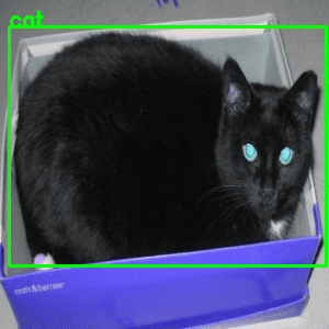
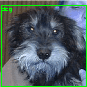
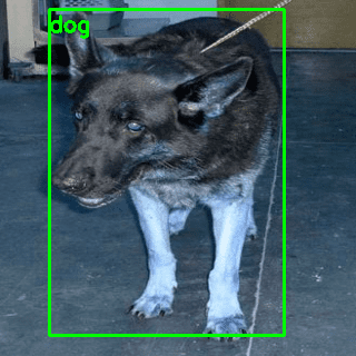
As we can see from the results, the pretrained YOLOv5 model localizes reasonably well on all the images.

Testing Custom Images on the SSD Model

For inference on the SSD model, we’ll follow a pattern similar to what was done in the YOLOv5 inference script.

# import the necessary packages
from pyimagesearch.data_utils import get_dataloader
from pyimagesearch.data_utils import normalize
from pyimagesearch import config
from torchvision.datasets import ImageFolder
from torch.utils.data import Subset
from sklearn.model_selection import train_test_split
from torchvision.transforms import Compose
from torchvision.transforms import ToTensor
from torchvision.transforms import Resize
import matplotlib.patches as patches
import matplotlib.pyplot as plt
import numpy as np
import random
import torch
import cv2
import os

# initialize test transform pipeline
testTransform = Compose([
	Resize((config.IMAGE_SIZE, config.IMAGE_SIZE)), ToTensor()])

# create the test dataset and initialize the test data loader
testDataset = ImageFolder(config.TEST_PATH, testTransform)
testLoader = get_dataloader(testDataset, config.PRED_BATCH_SIZE)

# initialize iterable variable
sweeper = iter(testLoader)

# list to store permuted images
imageInput = []

As earlier, we create the PyTorch Transform instance on Lines 20 and 21. Then, using the ImageFolder utility function, we create the dataset instance as required, followed by the Dataloader instance on Lines 24 and 25.

The iterable variable sweeper is initialized on Line 28 for ease of access to the test data. Next, to store images that we will preprocess, we initialize a list called imageInput (Line 31).

# grab a batch of test data
print("[INFO] getting the test data...")
batch = next(sweeper)
(images, _ ) = (batch[0], batch[1])

# switch off autograd
with torch.no_grad():
	# send the images to the device
	images = images.to(config.DEVICE) 
 
	# loop over all the batch 
	for index in range(0, config.PRED_BATCH_SIZE):
		# grab the image, de-normalize it, scale the raw pixel
		# intensities to the range [0, 255], and change the channel
		# ordering from channels first tp channels last
		image = images[index]
		image = image.permute((1, 2, 0))
		imageInput.append(image.cpu().detach().numpy())

The process shown in the above code block is again repeated from the YOLOv5 inference script. We grab a batch of data (Lines 35 and 36) and loop over them to rearrange each to channel-last and append them to our imageInput list (Lines 39-50).

# call the required entry points
ssdModel = torch.hub.load("NVIDIA/DeepLearningExamples:torchhub",
	"nvidia_ssd")
utils = torch.hub.load("NVIDIA/DeepLearningExamples:torchhub", 
	"nvidia_ssd_processing_utils")

# flash model to the device and set it to eval mode
ssdModel.to(config.DEVICE)
ssdModel.eval()

# new list for processed input
processedInput = []

# loop over images and preprocess them
for image in imageInput:
	image = normalize (image)
	processedInput.append(image)

# convert the preprocessed images into tensors
inputTensor = utils.prepare_tensor(processedInput)

On Lines 53 and 54, we use the torch.hub.load function to:

• Call the SSD model by evoking its corresponding repository and entry point name
• Call an additional Utility function to help preprocess the input images according to the SSD model’s need.

The model is then loaded to our device in use and set to evaluation mode (Lines 59 and 60).

On Line 63, we create an empty list to keep the preprocessed input. Then, looping over the images, we normalize each of them and append them accordingly (Lines 66-68). Finally, to convert the preprocessed images to required tensors, we use a previously called utility function (Lines 71).

# turn off auto-grad
print("[INFO] getting detections from the test data...")
with torch.no_grad():
	# feed images to model
	detections = ssdModel(inputTensor)

# decode the results and filter them using the threshold
resultsPerInput = utils.decode_results(detections)
bestResults = [utils.pick_best(results,
	config.THRESHOLD) for results in resultsPerInput]

Switching off automatic gradients, feed the image tensors to the SSD model (Lines 75-77).

On Line 80, we use another function from utils called decode_results to get all the results corresponding to each input image. Now, since SSD gives you 8732 detections, we’ll use the threshold confidence value previously set in the config.py script to keep only the ones with more than 50% confidence (Lines 81 and 82).

That would mean that the bestResults list contains bounding box values, object classes, and confidence values corresponding to each image it encountered while it gave its detection outputs. This way, the index of this list will directly correspond to the index of our input list.

# get coco labels 
classesToLabels = utils.get_coco_object_dictionary()

# loop over the image batch
for image_idx in range(len(bestResults)):
	(fig, ax) = plt.subplots(1)

	# denormalize the image and plot the image
	image = processedInput[image_idx] / 2 + 0.5
	ax.imshow(image)

	# grab bbox, class, and confidence values
	(bboxes, classes, confidences) = bestResults[image_idx]

Since we don’t have a way to decode the class integer results to their corresponding labels, we’ll take the help of yet another function from utils called get_coco_object_dictionary (Line 85).

The next step is to match the results to their corresponding images and plot the bounding box on them. Accordingly, grab the corresponding image using the image index and denormalize it (Lines 88-93).

Using the same index, we grab the bounding box results, class name, and confidence values from the results (Line 96).

	# loop over the detected bounding boxes
	for idx in range(len(bboxes)):
		# scale values up according to image size
		(left, bot, right, top) = bboxes[idx ] * 300

		# draw the bounding box on the image
		(x, y, w, h) = [val for val in [left, bot, right - left,
			top - bot]]
		rect = patches.Rectangle((x, y), w, h, linewidth=1,
			edgecolor="r", facecolor="none")
		ax.add_patch(rect)
		ax.text(x, y,
			"{} {:.0f}%".format(classesToLabels[classes[idx] - 1],
			confidences[idx] * 100),
			bbox=dict(facecolor="white", alpha=0.5))

Since there can be multiple detections for a single image, we create a loop and start iterating over the available bounding boxes (Line 99). The bounding box results are in the range of 0 and 1. So it’s important to scale them according to the image height and width when unpacking the bounding box values (Line 101).

Now, the SSD model outputs the left, bottom, right, and top coordinates instead of the YOLOv5s starting X, starting Y, ending X, and ending Y values. So, we have to calculate the starting X, starting Y, width, and height to plot the rectangle on the image (Lines 104-107).

Finally, we add the object class name with the help of the classesToLabels function on Lines 109-112.

# check to see if the output directory already exists, if not
# make the output directory
if not os.path.exists(config.SSD_OUTPUT):
    os.makedirs(config.SSD_OUTPUT)

# save plots to output directory
print("[INFO] saving the inference...")
outputFileName = os.path.join(config.SSD_OUTPUT, "output.png")
plt.savefig(outputFileName)

We end the script with our image plotted by saving the output image file to our previously set location (Lines 121 and 120).

Let’s see the script in action!

In Figures 9-11, we have the bounding boxes predicted by the SSD model on images from our custom dataset.

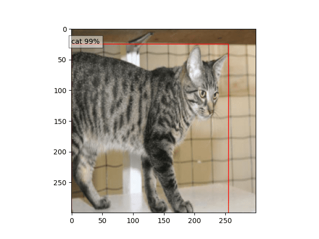
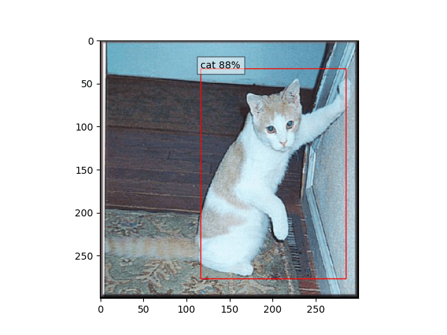
It’s commendable how in Figure 11, the SSD model managed to figure out the puppy, which has almost camouflaged itself with its parent. Otherwise, the SSD model performed reasonably well on most images, with the confidence values telling us how sure it is of its predictions.

Summary

Since Object Detection has become a major part of our lives, having access to models that can replicate high-level research/industry-level results is a huge boon for the learning crowd.

Torch Hub’s simple yet stellar system of entry point calling is again displayed in this tutorial, where we can call the pretrained all-powerful models and their auxiliary helper functions to help us pre-process our data better. The beauty of this whole process is that if the model owners decide to push a change to their repository, instead of going through many processes to change hosted data, they need to push their changes into their repository itself.

With the whole process of dealing with hosted data simplified, PyTorch has hit a home run with their whole process of collaboration with GitHub. This way, even us users who call the models can learn more about it in the repositories themselves since it would have to be public.

I hope this tutorial served as a good starting point on using these models for your custom tasks. Readers are instructed to try out their images or think about using these models for their custom tasks!

Citation Information

Chakraborty, D. “Torch Hub Series #3: YOLOv5 and SSD — Models on Object Detection,” PyImageSearch, 2022, https://pyimagesearch.com/2022/01/03/torch-hub-series-3-yolov5-ssd-models-on-object-detection/

@article{dev_2022_THS3,
  author = {Devjyoti Chakraborty},
  title = {{Torch Hub} Series \#3: {YOLOv5} and {SSD} — Models on Object Detection},
  journal = {PyImageSearch},
  year = {2022},
  note = {https://pyimagesearch.com/2022/01/03/torch-hub-series-3-yolov5-and-ssd-models-on-object-detection/},
}

To download the source code to this post (and be notified when future tutorials are published here on PyImageSearch), simply enter your email address in the form below!