OpenCV Morphological Operations

In this tutorial, you will learn about applying morphological operations with OpenCV.

The morphological operations we’ll be covering include:

• Erosion
• Dilation
• Opening
• Closing
• Morphological gradient
• Black hat
• Top hat (also called “White hat”)

These image processing operations are applied to grayscale or binary images and are used for preprocessing for OCR algorithms, detecting barcodes, detecting license plates, and more.

And sometimes a clever use of morphological operations can allow you to avoid more complicated (and computationally expensive) machine learning and deep learning algorithms.

As a serious computer vision practitioner, you need to understand morphological operations.

To learn how to apply morphological operations with OpenCV, just keep reading.

OpenCV Morphological Operations

Morphological operations are simple transformations applied to binary or grayscale images. More specifically, we apply morphological operations to shapes and structures inside of images.

We can use morphological operations to increase the size of objects in images as well as decrease them. We can also utilize morphological operations to close gaps between objects as well as open them.

Morphological operations “probe” an image with a structuring element. This structuring element defines the neighborhood to be examined around each pixel. And based on the given operation and the size of the structuring element we are able to adjust our output image.

This explanation of a structuring element may sound vague — that’s because it is. There are many different morphological transformations that perform “opposite” operations from one another — just as addition is the “opposite” of subtraction, we can think of the erosion morphological operation as the “opposite” of dilation.

If this sounds confusing, don’t worry — we’ll be reviewing many examples of each of these morphological transformations, and by the time you are done reading through this tutorial, you’ll have a crystal clear view of morphological operations.

Why learn about morphological operations?

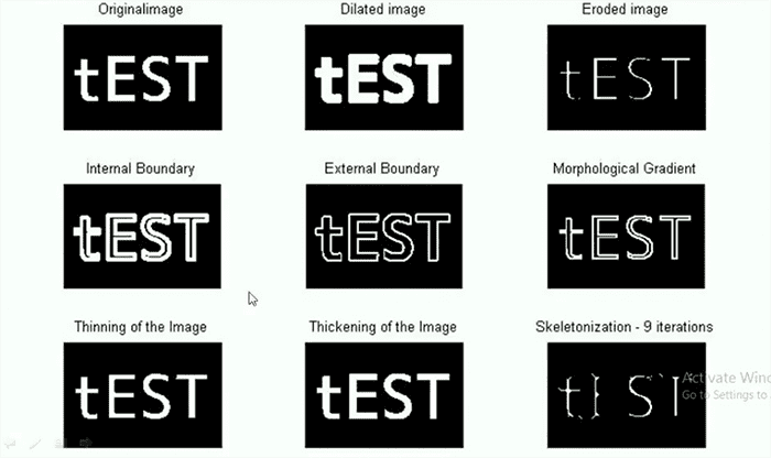
Morphological operations are one of my favorite topics to cover in image processing.

Why is that?

Because these transformations are so powerful.

Oftentimes I see computer vision researchers and developers trying to solve a problem and immediately dive into advanced computer vision, machine learning, and deep learning techniques. It seems that once you learn to wield a hammer, every problem looks like a nail.

However, there are times where a more “elegant” solution can be found using less advanced techniques. Sure, these techniques may not be floating around on a cloud of buzzwords for the latest state-of-the-art algorithms, but they can get the job done.

For instance, I once wrote an article on the PyImageSearch blog on detecting barcodes in images. I didn’t use any fancy techniques. I didn’t use any machine learning. In fact, I was able to detect barcodes in images using nothing more than the introductory topics we’ve discussed so far in this series.

Crazy, isn’t it?

But seriously, pay attention to these transformations — there will be times in your computer vision career when you’ll be ready to swing your hammer down on a problem, only to realize that a more elegant, simple solution may already exist. And more than likely, you may find that elegant solution in morphological operations.

Let’s go ahead and get started by discussing the component that makes morphological operations possible: the structuring element.

The concept of “structuring elements”

Remember back in our tutorial on image kernels and convolutions?

Well, you can (conceptually) think of a structuring element as a type of kernel or mask. However, instead of applying a convolution, we are only going to perform simple tests on the pixels.

And just like in image kernels, the structuring element slides from left-to-right and top-to-bottom for each pixel in the image. Also just like kernels, structuring elements can be of arbitrary neighborhood sizes.

For example, let’s take a look at the 4-neighborhood and 8-neighborhood of the central pixel red below:

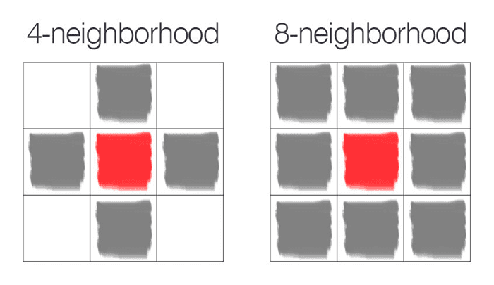
Here, we can see that the central pixel (i.e., the red pixel) is located at the center of the neighborhood:

• The 4-neighborhood (left) defines the region surrounding the central pixel as the pixels to the north, south, east, and west.
• The 8-neighborhood (right) extends this region to include the corner pixels as well

This is just an example of two simple structuring elements. But we could also make them arbitrary rectangle or circular structures as well — it all depends on your particular application.

In OpenCV, we can either use the cv2.getStructuringElement function or NumPy itself to define our structuring element. Personally, I prefer to use the cv2.getStructuringElement function since it gives you more control over the returned element, but again, that is a personal choice.

If the concept of structuring elements is not entirely clear, that’s okay. We’ll be reviewing many examples of them inside this lesson. For the time being, understand that a structuring element behaves similar to a kernel or a mask — but instead of convolving the input image with our structuring element, we’re instead only going to be applying simple pixel tests.

Now that we have a basic understanding of structuring elements, let’s configure our development environment, review the project directory structure, and then write some code.

Configuring your development environment

To follow this guide, you need to have the OpenCV library installed on your system.

Luckily, OpenCV is pip-installable:

$ pip install opencv-contrib-python

If you need help configuring your development environment for OpenCV, I highly recommend that you read my pip install OpenCV guide — it will have you up and running in a matter of minutes.

Having problems configuring your development environment?

All that said, are you:

• Short on time?
• Learning on your employer’s administratively locked system?
• Wanting to skip the hassle of fighting with the command line, package managers, and virtual environments?
• Ready to run the code right now on your Windows, macOS, or Linux system?

Then join PyImageSearch University today!

Gain access to Jupyter Notebooks for this tutorial and other PyImageSearch guides that are pre-configured to run on Google Colab’s ecosystem right in your web browser! No installation required.

And best of all, these Jupyter Notebooks will run on Windows, macOS, and Linux!

Project structure

Before we can start implementing morphological operations with OpenCV, let’s first review our project directory structure.

Start by accessing the “Downloads” section of this tutorial to retrieve the source code and example images:

$ tree . --dirsfirst
.
├── car.png
├── morphological_hats.py
├── morphological_ops.py
├── pyimagesearch_logo.png
└── pyimagesearch_logo_noise.png

0 directories, 5 files

We have two Python scripts to to review today:

1. morphological_ops.py: Applies OpenCV’s morphological operations, including erosion, dilation, opening, closing, and morphological gradient.
2. morphological_hats.py: Applies a black hat and top hat/white hat operation with OpenCV.

The three .png images included in our project structure will be utilized by these two scripts to demonstrate various morphological operations.

Erosion

Just like water rushing along a river bank erodes the soil, an erosion in an image “erodes” the foreground object and makes it smaller. Simply put, pixels near the boundary of an object in an image will be discarded, “eroding” it away.

Erosion works by defining a structuring element and then sliding this structuring element from left-to-right and top-to-bottom across the input image.

A foreground pixel in the input image will be kept only if all pixels inside the structuring element are > 0. Otherwise, the pixels are set to 0 (i.e., background).

Erosion is useful for removing small blobs in an image or disconnecting two connected objects.

We can perform erosion by using the cv2.erode function. Let’s open a new file, name it morphological.py_ops.py, and start coding:

# import the necessary packages
import argparse
import cv2

# construct the argument parser and parse the arguments
ap = argparse.ArgumentParser()
ap.add_argument("-i", "--image", required=True,
	help="path to input image")
args = vars(ap.parse_args())

Lines 2 and 3 import argparse (for command line arguments) and cv2 (our OpenCV bindings).

We only have a single command line argument to parse, our input --image that we’ll be applying erosions to.

In most examples in this lesson we’ll be applying morphological operations to the PyImageSearch logo, which we can see below:

As I mentioned earlier in this lesson, we typically (but not always) apply morphological operations to binary images. As we’ll see later in this lesson, there are exceptions to that, especially when using the black hat and white hat operators, but for the time being, we are going to assume we are working with a binary image, where the background pixels are black and the foreground pixels are white.

Let’s load our input --image from disk and then apply a series of erosions:

# load the image, convert it to grayscale, and display it to our
# screen
image = cv2.imread(args["image"])
gray = cv2.cvtColor(image, cv2.COLOR_BGR2GRAY)
cv2.imshow("Original", image)

# apply a series of erosions
for i in range(0, 3):
	eroded = cv2.erode(gray.copy(), None, iterations=i + 1)
	cv2.imshow("Eroded {} times".format(i + 1), eroded)
	cv2.waitKey(0)

Line 13 loads our input image from disk while Line 14 converts it to grayscale. Since our image is already pre-segmented, we are now working with a binary image.

Given our logo image, we apply a series of erosions on Lines 18-21. The for loop controls the number of times, or iterations, we are going to apply the erosion. As the number of erosions increases, the foreground logo will start to “erode” and disappear.

We perform the actual erosion on Line 19 by making a call to the cv2.erode function. This function takes two required arguments and a third optional one.

The first argument is the image that we want to erode — in this case, it’s our binary image (i.e., the PyImageSearch logo).

The second argument to cv2.erode is the structuring element. If this value is None, then a 3×3 structuring element, identical to the 8-neighborhood structuring element we saw above will be used. Of course, you could supply your own custom structuring element here instead of None as well.

The last argument is the number of iterations the erosion is going to be performed. As the number of iterations increases, we’ll see more and more of the PyImageSearch logo eaten away.

Finally, Line 20 and 21 show us our eroded image.

When you execute this script you’ll see the following output from our erosion operations:

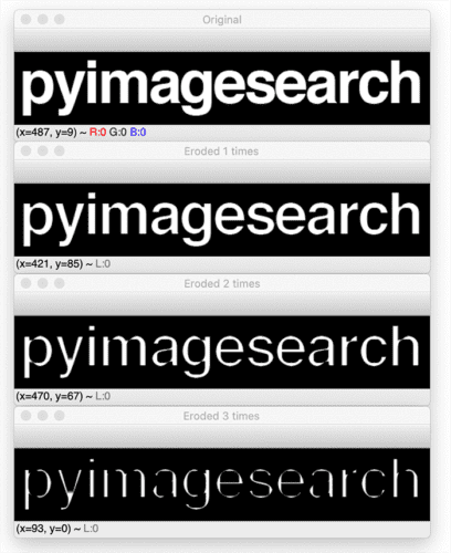
On the very top we have our original image. And then underneath the image, we have the logo being eroded a total of 1, 2, and 3 times, respectively. Notice as the number of erosion iterations increases, more and more of the logo is eaten away.

Again, erosions are most useful for removing small blobs from an image or disconnecting two connected components. With this in mind, take a look at the letter “p” in the PyImageSearch logo. Notice how the circular region of the “p” has disconnected from the stem after 2 erosions — this is an example of disconnecting two connected components of an image.

Dilation

The opposite of an erosion is a dilation. Just like an erosion will eat away at the foreground pixels, a dilation will grow the foreground pixels.

Dilations increase the size of foreground objects and are especially useful for joining broken parts of an image together.

Dilations, just as an erosion, also utilize structuring elements — a center pixel p of the structuring element is set to white if ANY pixel in the structuring element is > 0.

We apply dilations using the cv2.dilate function:

# close all windows to cleanup the screen
cv2.destroyAllWindows()
cv2.imshow("Original", image)

# apply a series of dilations
for i in range(0, 3):
	dilated = cv2.dilate(gray.copy(), None, iterations=i + 1)
	cv2.imshow("Dilated {} times".format(i + 1), dilated)
	cv2.waitKey(0)

Lines 24 and 25 simply close all open windows and display our original image to give us a fresh start.

Line 28 then starts looping over the number of iterations, just as we did with the cv2.erode function.

The actual dilation is performed on Line 29 by making a call to the cv2.dilate function, where the actual function signature is identical to that of cv2.erode.

The first argument is the image we want to dilate; the second is our structuring element, which when set to None is a 3×3 8-neighborhood structuring element; and the final argument is the number of dilation iterations we are going to apply.

The output of our dilation can be seen below:

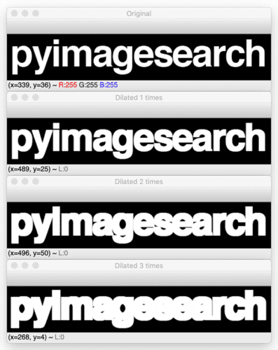
Again, at the very top we have our original input image. And below the input image we have our image dilated 1, 2, and 3 times, respectively.

Unlike an erosion where the foreground region is slowly eaten away at, a dilation actually grows our foreground region.

Dilations are especially useful when joining broken parts of an object — for example, take a look at the bottom image where we have applied a dilation with 3 iterations. By this point, the gaps between all letters in the logo have been joined.

Opening

An opening is an erosion followed by a dilation.

Performing an opening operation allows us to remove small blobs from an image: first an erosion is applied to remove the small blobs, then a dilation is applied to regrow the size of the original object.

Let’s look at some example code to apply an opening to an image:

# close all windows to cleanup the screen, then initialize a list of
# of kernels sizes that will be applied to the image
cv2.destroyAllWindows()
cv2.imshow("Original", image)
kernelSizes = [(3, 3), (5, 5), (7, 7)]

# loop over the kernels sizes
for kernelSize in kernelSizes:
	# construct a rectangular kernel from the current size and then
	# apply an "opening" operation
	kernel = cv2.getStructuringElement(cv2.MORPH_RECT, kernelSize)
	opening = cv2.morphologyEx(gray, cv2.MORPH_OPEN, kernel)
	cv2.imshow("Opening: ({}, {})".format(
		kernelSize[0], kernelSize[1]), opening)
	cv2.waitKey(0)

Lines 35 and 36 perform cleanup by closing all open windows and re-displaying our original image.

Take a look at the new variable we are defining on Line 37, kernelSizes. This variable defines the width and height, respectively, of the structuring element we are going to apply.

We loop over each of these kernelSizes on Line 40 and then make a call to cv2.getStructuringElement on Line 43 to build our structuring element.

The cv2.getStructuringElement function requires two arguments: the first is the type of structuring element we want, and the second is the size of the structuring element (which we grab from the for loop on Line 40).

We pass in a value of cv2.MORPH_RECT to indicate that we want a rectangular structuring element. But you could also pass in a value of cv2.MORPH_CROSS to get a cross shape structuring element (a cross is like a 4-neighborhood structuring element, but can be of any size), or cv2.MORPH_ELLIPSE to get a circular structuring element.

Exactly which structuring element you use is dependent upon your application — and I’ll leave it as an exercise to the reader to play with each of these structuring elements.

The actual opening operation is performed on Line 42 by making a call to the cv2.morphologyEx function. This function is abstract in a sense — it allows us to pass in whichever morphological operation we want, followed by our kernel/structuring element.

The first required argument of cv2.morphologyEx is the image we want to apply the morphological operation to. The second argument is the actual type of morphological operation — in this case, it’s an opening operation. The last required argument is the kernel/structuring element that we are using.

Finally, Lines 45-47 display the output of applying our opening.

As I mentioned above, an opening operation allows us to remove small blobs in an image. I went ahead and added some blobs to the PyImageSearch logo (pyimagesearch_logo_noise.png in our project directory structure):

When you apply our opening morphological operations to this noisy image you’ll receive the following output:

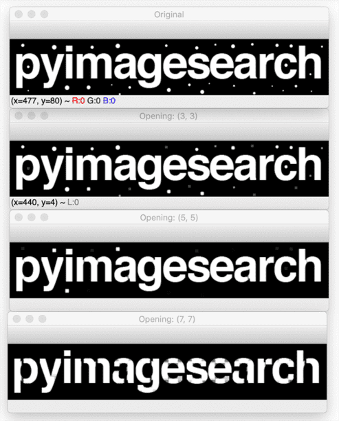
Notice how by the time we are using a kernel of size 5×5, the small, random blobs are nearly completely gone. And by the time it reaches a kernel of size 7×7, our opening operation has not only removed all the random blobs, but also “opened” holes in the letter “p” and the letter “a”.

Closing

The exact opposite to an opening would be a closing. A closing is a dilation followed by an erosion.

As the name suggests, a closing is used to close holes inside of objects or for connecting components together.

The below code block contains the code to perform a closing:

# close all windows to cleanup the screen
cv2.destroyAllWindows()
cv2.imshow("Original", image)

# loop over the kernels sizes again
for kernelSize in kernelSizes:
	# construct a rectangular kernel form the current size, but this
	# time apply a "closing" operation
	kernel = cv2.getStructuringElement(cv2.MORPH_RECT, kernelSize)
	closing = cv2.morphologyEx(gray, cv2.MORPH_CLOSE, kernel)
	cv2.imshow("Closing: ({}, {})".format(
		kernelSize[0], kernelSize[1]), closing)
	cv2.waitKey(0)

Performing the closing operation is again accomplished by making a call to cv2.morphologyEx, but this time we are going to indicate that our morphological operation is a closing by specifying the cv2.MORPH_CLOSE flag.

We’ll go back to using our original image (without the random blobs). The output for applying a closing operation with increasing structuring element sizes can be seen below:

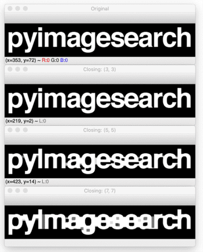
Notice how the closing operation is starting to bridge the gap between letters in the logo. Furthermore, letters such as “e”, “s”, and “a” are practically filled in.

Morphological gradient

A morphological gradient is the difference between a dilation and erosion. It is useful for determining the outline of a particular object of an image:

# close all windows to cleanup the screen
cv2.destroyAllWindows()
cv2.imshow("Original", image)

# loop over the kernels a final time
for kernelSize in kernelSizes:
	# construct a rectangular kernel and apply a "morphological
	# gradient" operation to the image
	kernel = cv2.getStructuringElement(cv2.MORPH_RECT, kernelSize)
	gradient = cv2.morphologyEx(gray, cv2.MORPH_GRADIENT, kernel)
	cv2.imshow("Gradient: ({}, {})".format(
		kernelSize[0], kernelSize[1]), gradient)
	cv2.waitKey(0)

The most important line to pay attention to is Line 72, where we make a call to cv2.morphologyEx — but this time we supply the cv2.MORPH_GRADIENT flag to indicate that we want to apply the morphological gradient operation to reveal the outline of our logo:

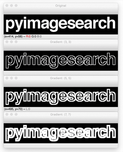
Notice how the outline of the PyImageSearch logo has been clearly revealed after applying the morphological gradient operation.

Top hat/white hat and black hat

A top hat (also known as a white hat) morphological operation is the difference between the original (grayscale/single channel) input image and the opening.

A top hat operation is used to reveal bright regions of an image on dark backgrounds.

Up until this point we have only applied morphological operations to binary images. But we can also apply morphological operations to grayscale images as well. In fact, both the top hat/white hat and the black hat operators are more suited for grayscale images rather than binary ones.

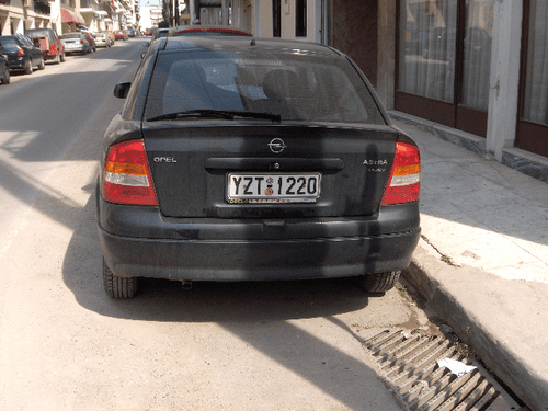
To demonstrate applying morphological operations, let’s take a look at the following image where our goal is to detect the license plate region of the car:

So how are we going to go about doing this?

Well, taking a look at the example image above, we see that the license plate is bright since it’s a white region against a dark background of the car itself. An excellent starting point to finding the region of a license plate would be to use the top hat operator.

To test out the top hat operator, create a new file, name it morphological_hats.py, and insert the following code:

# import the necessary packages
import argparse
import cv2

# construct the argument parser and parse the arguments
ap = argparse.ArgumentParser()
ap.add_argument("-i", "--image", required=True,
	help="path to input image")
args = vars(ap.parse_args())

Lines 2 and 3 import our required Python packages while Lines 6-9 parse our command line arguments. We only need a single argument, --image, the path to our input image (which we presume to be car.png in our project structure).

Let’s load our input --image from disk:

# load the image and convert it to grayscale
image = cv2.imread(args["image"])
gray = cv2.cvtColor(image, cv2.COLOR_BGR2GRAY)

# construct a rectangular kernel (13x5) and apply a blackhat
# operation which enables us to find dark regions on a light
# background
rectKernel = cv2.getStructuringElement(cv2.MORPH_RECT, (13, 5))
blackhat = cv2.morphologyEx(gray, cv2.MORPH_BLACKHAT, rectKernel)

Lines 12 and 13 laid our input image from disk and convert it to grayscale, thereby preparing it for our black hat and white hat operations.

Line 18 then defines a rectangular structuring element with a width of 13 pixels and a height of 5 pixels. As I mentioned earlier in this lesson, structuring elements can be of arbitrary size. And in this case, we are applying a rectangular element that is almost 3x wider than it is tall.

And why is this?

Because a license plate is roughly 3x wider than it is tall!

By having some basic a priori knowledge of the objects you want to detect in images, we can construct structuring elements to better aid us in finding them.

Line 19 applies the black hat operator.

In a similar fashion we can also apply a top hat/white hat operation:

# similarly, a tophat (also called a "whitehat") operation will
# enable us to find light regions on a dark background
tophat = cv2.morphologyEx(gray, cv2.MORPH_TOPHAT, rectKernel)

# show the output images
cv2.imshow("Original", image)
cv2.imshow("Blackhat", blackhat)
cv2.imshow("Tophat", tophat)
cv2.waitKey(0)

To specify a top hat/white hat operator instead of a blackhat, we simply change the type of operator to cv2.MORPH_TOPHAT.

Below you can see the output of applying the top hat operators:

Notice how the right (i.e., the top hat/white hat) regions that are light against a dark background are clearly displayed — in this case, we can clearly see that the license plate region of the car has been revealed.

But also note that the license plate characters themselves have not been included. This is because the license plate characters are dark against a light background.

To help remedy that, we can apply a black hat operator:

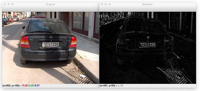
To reveal our license plate characters you would first segment out the license plate itself via a top hat operator and then apply a black hat operator (or thresholding) to extract the individual license plate characters (perhaps using methods like contour detection).

Running our morphological operations demos

To run our morphological operation demos, be sure to access the “Downloads” section of this tutorial to retrieve the source code and example images.

You can execute the morphological_ops.py script using this command:

$ python morphological_ops.py --image pyimagesearch_logo.png

And the morphological_hats.py script can be started by using this command:

$ python morphological_hats.py --image car.png

The output of these scripts should match the images and figures I have provided above.

Summary

In this tutorial, we learned that morphological operations are image processing transformations applied to either grayscale or binary images. These operations require a structuring element, which is used to define the neighborhood of pixels the operation is applied to.

We also reviewed the most important morphological operations that you’ll use inside your own applications:

• Erosion
• Dilation
• Opening
• Closing
• Morphological gradient
• Top hat/white hat
• Black hat

Morphological operations are commonly used as pre-processing steps to more powerful computer vision solutions such as OCR, Automatic Number Plate Recognition (ANPR), and barcode detection.

While these techniques are simple, they are actually extremely powerful and tend to be highly useful when pre-processing your data. Do not overlook them.

To download the source code to this post (and be notified when future tutorials are published here on PyImageSearch), simply enter your email address in the form below!