Face clustering with Python

Today’s blog post is inspired by a question from PyImageSearch reader, Leonard Bogdonoff.

After I published my previous post on Face recognition with OpenCV and deep learning, Leonard wrote in and asked:

Hey Adrian, can you go into identity clustering? I have a dataset of photos and I can’t seem to pinpoint how I would process them to identify the unique people.

Such an application of “face clustering” or “identity clustering” could be used to aid to law enforcement.

Consider a scenario where two perpetrators rob a bank in a busy city such as Boston or New York. The bank’s security cameras are working properly, capturing the robbery going down — but the criminals wear ski masks so you cannot see their faces.

The perpetrators flee the bank with the cash hidden under their clothes, taking off their masks, and dumping them in nearby trash can as to not appear “suspicious” in public.

Will they get away with the crime?

Maybe.

But security cameras installed at nearby gas stations, restaurants, and red lights/major intersections capture all pedestrian activity in the neighborhood.

After the police arrive their detectives could leverage face clustering to find all unique faces across all video feeds in the area — given the unique faces, detectives could: (1) manually investigate them and compare them to bank teller descriptions, (2) run an automated search to compare faces to a known database of criminals, or (3) apply good ole’ detective work and look for suspicious individuals.

This is a fictitious example of course, but I hope you see the value in how face clustering could be used in real-world situations.

To learn more about face clustering, and how to implement it using Python, and deep learning, just keep reading.

Face clustering with Python

Face recognition and face clustering are different, but highly related concepts. When performing face recognition we are applying supervised learning where we have both (1) example images of faces we want to recognize along with (2) the names that correspond to each face (i.e., the “class labels”).

But in face clustering we need to perform unsupervised learning — we have only the faces themselves with no names/labels. From there we need to identify and count the number of unique people in a dataset.

In the first part of this blog post, we’ll discuss our face clustering dataset and the project structure we’ll use for building the project.

From there I’ll help you write two Python scripts:

1. One to extract and quantify the faces in a dataset
2. And another to cluster the faces, where each resulting cluster (ideally) represents a unique individual

From there we’ll run our face clustering pipeline on a sample dataset and examine the results.

Configuring your development environment

In our previous face recognition post, I explained how to configure your development environment in the section titled “Install your face recognition libraries” — please be sure to refer to it when configuring your environment.

As a quick breakdown, here is everything you’ll need in your Python environment:

• OpenCV
• dlib
• face_recognition
• imutils
• scikit-learn

If you have a GPU, you’ll want to install dlib with CUDA bindings which is also described in this previous post.

Our face clustering dataset

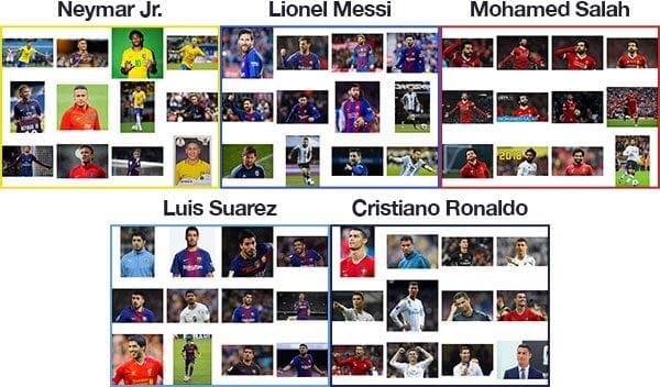
With the 2018 FIFA World Cup semi-finals starting tomorrow I thought it would be fun to apply face clustering to faces of famous soccer players.

As you can see from Figure 1 above, I have put together a dataset of five soccer players, including:

• Mohamed Salah
• Neymar Jr.
• Cristiano Ronaldo
• Lionel Messi
• Luis Suarez

In total, there are 129 images in the dataset.

Our goal will be to extract features quantifying each face in the image and cluster the resulting “facial feature vectors”. Ideally each soccer player will have their own respective cluster containing just their faces.

Face clustering project structure

Before we get started, be sure to grab the downloadable zip from the “Downloads” section of this blog post.

Our project structure is as follows:

$ tree --dirsfirst
.
├── dataset [129 entries]
│   ├── 00000000.jpg
│   ├── 00000001.jpg
│   ├── 00000002.jpg
│   ├── ...
│   ├── 00000126.jpg
│   ├── 00000127.jpg
│   └── 00000128.jpg
├── encode_faces.py
├── encodings.pickle
└── cluster_faces.py

1 directory, 132 files

Our project has one directory and three files:

• dataset/ : Contains 129 pictures of our five soccer players. Notice in the output above that there is no identifying information in the filenames or another file that identifies who is in each image. It would be impossible to know which soccer player is in which image based on filenames alone. We’re going to devise a face clustering algorithm to identify the similar and unique faces in the dataset.
• encode_faces.py : This is our first script — it computes face embeddings for all faces in the dataset and outputs a serialized encodings file.
• encodings.pickle : Our face embeddings serialized pickle file.
• cluster_faces.py : The magic happens in this script where we’ll cluster similar faces and ideally find the outliers.

Encoding faces via deep learning

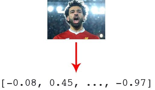
Before we can cluster a set of faces we first need to quantify them. This process of quantifying the face will be accomplished using a deep neural network responsible for:

• Accepting an input image
• And outputting a 128-d feature vector that quantifies the face

I discuss how this deep neural network works and how it was trained in my previous face recognition post, so be sure to refer to it if you have any questions on the network itself. Our encode_faces.py script will contain all code used to extract a 128-d feature vector representation for each face.

To see how this process is performed, create a file named encode_faces.py , and insert the following code:

# import the necessary packages
from imutils import paths
import face_recognition
import argparse
import pickle
import cv2
import os

# construct the argument parser and parse the arguments
ap = argparse.ArgumentParser()
ap.add_argument("-i", "--dataset", required=True,
	help="path to input directory of faces + images")
ap.add_argument("-e", "--encodings", required=True,
	help="path to serialized db of facial encodings")
ap.add_argument("-d", "--detection-method", type=str, default="cnn",
	help="face detection model to use: either `hog` or `cnn`")
args = vars(ap.parse_args())

Our required packages are imported on Lines 2-7. Take note of:

• paths from my imutils package
• face_recognition by Adam Geitgey, a PyImageConf2018 speaker

From there, we’ll parse our command line arguments on Lines 10-17:

• --dataset : The path to the input directory of faces and images.
• --encodings : The path to our output serialized pickle file containing the facial encodings.
• --detection-method : You may use either a Convolutional Neural Network (CNN) or Histogram of Oriented Gradients (HOG) method to detect the faces in an input image prior to quantifying the face. The CNN method is more accurate (but slower) whereas the HOG method is faster (but less accurate).

If you’re unfamiliar with command line arguments and how to use them, please refer to my previous post.

I’ll also mention that if you think this script is running slow or you would like to run the face clustering post in real-time without a GPU you should absolutely be setting --detection-method to hog instead of cnn . While the CNN face detector is more accurate, it’s far too slow to run in real-time without a GPU.

Let’s grab the paths to all the images in our input dataset:

# grab the paths to the input images in our dataset, then initialize
# out data list (which we'll soon populate)
print("[INFO] quantifying faces...")
imagePaths = list(paths.list_images(args["dataset"]))
data = []

On Line 22, we create a list of all imagePaths in our dataset using the dataset path provided in our command line argument.

From there, we initialize our data list which we’ll later populate with the image path, bounding box, and face encoding.

Let’s begin looping over all of the imagePaths :

# loop over the image paths
for (i, imagePath) in enumerate(imagePaths):
	# load the input image and convert it from RGB (OpenCV ordering)
	# to dlib ordering (RGB)
	print("[INFO] processing image {}/{}".format(i + 1,
		len(imagePaths)))
	print(imagePath)
	image = cv2.imread(imagePath)
	rgb = cv2.cvtColor(image, cv2.COLOR_BGR2RGB)

On Line 26, we begin our loop over the imagePaths and proceed to load the image (Line 32). Then we swap color channels in the image because dlib assumes rgb ordering rather than OpenCV’s default BGR. (Line 33).

Now that the image has been processed, let’s detect all the faces and grab their bounding box coordinates:

	# detect the (x, y)-coordinates of the bounding boxes
	# corresponding to each face in the input image
	boxes = face_recognition.face_locations(rgb,
		model=args["detection_method"])

We must detect the actual location of a face in an image before we can quantify it. This detection takes place on Lines 37 and 38. You’ll notice that the face_recognition API is very easy to use.

Note: We are using the CNN face detector for higher accuracy, but it will take a significantly longer time to run if you are using a CPU rather than a GPU. If you want the encoding script to run faster or your system, and your system does not have enough RAM or CPU power for the CNN face detector, use the HOG + Linear SVM method instead.

Let’s get to the “meat” of this script. In the next block, we’ll compute the facial encodings:

	# compute the facial embedding for the face
	encodings = face_recognition.face_encodings(rgb, boxes)

	# build a dictionary of the image path, bounding box location,
	# and facial encodings for the current image
	d = [{"imagePath": imagePath, "loc": box, "encoding": enc}
		for (box, enc) in zip(boxes, encodings)]
	data.extend(d)

Here, we compute the 128-d face encodings for each detected face in the rgb image (Line 41).

For each of the detected faces + encodings, we build a dictionary (Lines 45 and 46) that includes:

1. The path to the input image
2. The location of the face in the image (i.e., the bounding box)
3. The 128-d encoding itself

Then we add the dictionary to our data list (Line 47). We’ll use this information later when we want to visualize which faces belong to which cluster.

To close out this script, we simply write the data list to a serialized pickle file:

# dump the facial encodings data to disk
print("[INFO] serializing encodings...")
f = open(args["encodings"], "wb")
f.write(pickle.dumps(data))
f.close()

Using our command line argument, args["encodings"] , as the path + filename, we write the data list to disk as a serialized pickle file (Line 51-53).

Running the face encoding script

Before proceeding, scroll to the “Downloads” section to download code + images. You may elect to use your own dataset of images — that’s totally fine too, just be sure to provide the appropriate path in the command line arguments.

Then, open a terminal and activate your Python virtual environment (if you are using one) containing the libraries and packages you installed earlier in this post.

From there, using two command line arguments, execute the script to encode faces of famous soccer/futbol players as I’ve done below:

$ python encode_faces.py --dataset dataset --encodings encodings.pickle
[INFO] quantifying faces...
[INFO] processing image 1/129
dataset/00000038.jpg
[INFO] processing image 2/129
dataset/00000010.jpg
[INFO] processing image 3/129
dataset/00000004.jpg
...
[INFO] processing image 127/129
dataset/00000009.jpg
[INFO] processing image 128/129
dataset/00000021.jpg
[INFO] processing image 129/129
dataset/00000035.jpg
[INFO] serializing encodings...

This process can take a while and you can track the progress with the terminal output.

If you’re working with a GPU it will execute in quickly — in the order of 1-2 minutes. Just be sure that you installed dlib with CUDA bindings to take advantage of your GPU (as I mentioned above and described in this post).

However, if you’re just executing the script on your laptop with a CPU, the script may take 20-30 minutes to run.

Clustering faces

Now that we have quantified and encoded all faces in our dataset as 128-d vectors, the next step is to cluster them into groups.

Our hope is that each unique individual person will have their own separate cluster.

The problem is, many clustering algorithms such as k-means and Hierarchical Agglomerative Clustering, require us to specify the number of clusters we seek ahead of time.

For this example we know there are only five soccer players — but in real-world applications you would likely have no idea how many unique individuals there are in a dataset.

Therefore, we need to use a density-based or graph-based clustering algorithm that can not only cluster the data points but can also determine the number of clusters as well based on the density of the data.

For face clustering I would recommend two algorithms:

1. Density-based spatial clustering of applications with noise (DBSCAN)
2. Chinese whispers clustering

We’ll be using DBSCAN for this tutorial as our dataset is relatively small. For truly massive datasets you should consider using the Chinese whispers algorithm as it’s linear in time.

The DBSCAN algorithm works by grouping points together that are closely packed in an N-dimensional space. Points that lie close together will be grouped together in a single cluster.

DBSCAN also naturally handles outliers, marking them as such if they fall in low-density regions where their “nearest neighbors” are far away.

Let’s go ahead and implement face clustering using DBSCAN.

Open up a new file, name it cluster_faces.py , and insert the following code:

# import the necessary packages
from sklearn.cluster import DBSCAN
from imutils import build_montages
import numpy as np
import argparse
import pickle
import cv2

# construct the argument parser and parse the arguments
ap = argparse.ArgumentParser()
ap.add_argument("-e", "--encodings", required=True,
	help="path to serialized db of facial encodings")
ap.add_argument("-j", "--jobs", type=int, default=-1,
	help="# of parallel jobs to run (-1 will use all CPUs)")
args = vars(ap.parse_args())

DBSCAN is built into scikit-learn. We import the DBSCAN implementation on Line 2.

We also import the build_montages module from imutils on Line 3. We’ll be using this function to build a “montage of faces” for each cluster. If you’re curious about image montages, be sure to check out my previous post on Image montages with OpenCV.

Our other imports should be fairly familiar on Lines 4-7.

Let’s parse two command line arguments:

• --encodings : The path to the encodings pickle file that we generated in our previous script.
• --jobs : DBSCAN is multithreaded and a parameter can be passed to the constructor containing the number of parallel jobs to run. A value of -1 will use all CPUs available (and is also the default for this command line argument).

Let’s load the face embeddings data:

# load the serialized face encodings + bounding box locations from
# disk, then extract the set of encodings to so we can cluster on
# them
print("[INFO] loading encodings...")
data = pickle.loads(open(args["encodings"], "rb").read())
data = np.array(data)
encodings = [d["encoding"] for d in data]

In this block we’ve:

• Loaded the facial encodings data from disk (Line 21).
• Organized the data as a NumPy array (Line 22).
• Extracted the 128-d encodings from the data , placing them in a list (Line 23).

Now we can cluster the encodings in the next code block:

# cluster the embeddings
print("[INFO] clustering...")
clt = DBSCAN(metric="euclidean", n_jobs=args["jobs"])
clt.fit(encodings)

# determine the total number of unique faces found in the dataset
labelIDs = np.unique(clt.labels_)
numUniqueFaces = len(np.where(labelIDs > -1)[0])
print("[INFO] # unique faces: {}".format(numUniqueFaces))

To cluster the encodings, we simply create a DBSCAN object and then fit the model on the encodings themselves (Lines 27 and 28).

It can’t get any easier than that!

Now let’s determine the unique faces found in the dataset!

Referring to Line 31, clt.labels_ contains the label ID for all faces in our dataset (i.e., which cluster each face belongs to). To find the unique faces/unique label IDs, we simply use NumPy’s unique function. The result is a list of unique labelIDs .

On Line 32 we count the numUniqueFaces . There could potentially be a value of -1 in labelIDs — this value corresponds to the “outlier” class where a 128-d embedding was too far away from any other clusters to be added to it. Such points are called “outliers” and could either be worth examining or simply discarding based on the application of face clustering.

In our case, we excluded negative labelIDs in this count because we know for a fact that our dataset only contains images of 5 people. Whether or not you make such assumptions is highly dependent on your project.

The goal of our next three code blocks is to generate face montages of the unique soccer/futbol players in our dataset.

We begin the process by looping over all of the unique labelIDs :

# loop over the unique face integers
for labelID in labelIDs:
	# find all indexes into the `data` array that belong to the
	# current label ID, then randomly sample a maximum of 25 indexes
	# from the set
	print("[INFO] faces for face ID: {}".format(labelID))
	idxs = np.where(clt.labels_ == labelID)[0]
	idxs = np.random.choice(idxs, size=min(25, len(idxs)),
		replace=False)

	# initialize the list of faces to include in the montage
	faces = []

On Lines 41-43 we find all the indexes for the current labelID and then grab a random sample of at most 25 images to include in the montage.

The faces list will include the face images themselves (Line 46). We’ll need another loop to populate this list:

	# loop over the sampled indexes
	for i in idxs:
		# load the input image and extract the face ROI
		image = cv2.imread(data[i]["imagePath"])
		(top, right, bottom, left) = data[i]["loc"]
		face = image[top:bottom, left:right]

		# force resize the face ROI to 96x96 and then add it to the
		# faces montage list
		face = cv2.resize(face, (96, 96))
		faces.append(face)

We begin looping over all idxs in our random sample on Line 49.

Inside the first part of the loop, we:

• Load the image from disk and extract the face ROI (Lines 51-53) using the bounding box coordinates found during our face embedding step.
• Resize the face to a fixed 96×96 (Line 57) so we can add it to the faces montage (Line 58) used to visualize each cluster.

To finish out our top-level loop, let’s build the montage and display it to the screen:

	# create a montage using 96x96 "tiles" with 5 rows and 5 columns
	montage = build_montages(faces, (96, 96), (5, 5))[0]
	
	# show the output montage
	title = "Face ID #{}".format(labelID)
	title = "Unknown Faces" if labelID == -1 else title
	cv2.imshow(title, montage)
	cv2.waitKey(0)

We employ the build_montages function of imutils to generate a single image montage containing a 5×5 grid of faces (Line 61).

From there, we title the window (Lines 64 and 65) followed by showing the montage in the window on our screen.

So long as the window opened by OpenCV is open, you can press a key to display the next face cluster montage.

Face clustering results

Be sure to use the “Downloads” section of this blog post to download the code and data necessary to run this script.

This script requires just one command line argument — the path to the encodings file. To perform face clustering for soccer/futbol players, just enter the following command in your terminal:

$ python cluster_faces.py --encodings encodings.pickle
[INFO] loading encodings...
[INFO] clustering...
[INFO] # unique faces: 5
[INFO] faces for face ID: -1
[INFO] faces for face ID: 0
[INFO] faces for face ID: 1
[INFO] faces for face ID: 2
[INFO] faces for face ID: 3
[INFO] faces for face ID: 4

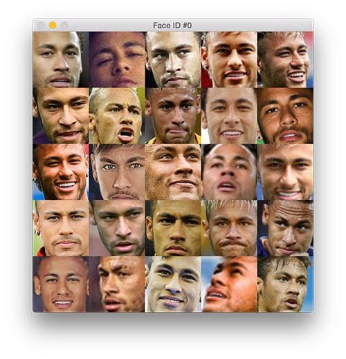
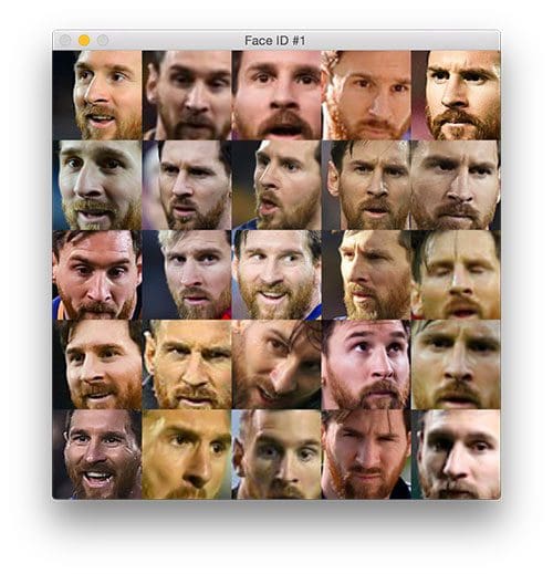
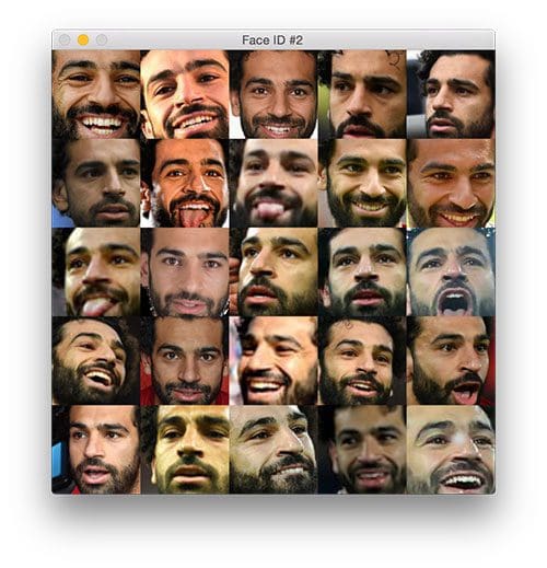
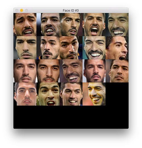
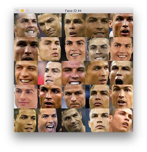
Five face cluster classes are identified. The face ID of -1 contains any outliers found. You’ll be presented with the cluster montage on your screen. To generate the next face cluster montage just press a key (with the window in focus so that OpenCV’s highgui module can capture your keypress).

Here are the face clusters generated from our 128-d facial embeddings and the DBSCAN clustering algorithm on our dataset:

And finally, the unknown faces are presented (it is actually displayed first, but I’m providing commentary here last):

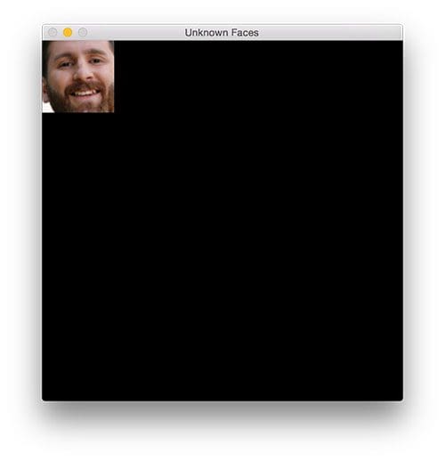
Out of the 129 images of 5 people in our dataset, only a single face is not grouped into an existing cluster (Figure 8; Lionel Messi).

Our unsupervised learning DBSCAN approach generated five clusters of data. Unfortunately, a single image of Lionel Messi wasn’t clustered with the other pictures of him, but overall this method worked quite well.

This same approach we used today can be used to cluster faces in your own applications.

Summary

In today’s blog post you learned how to perform face clustering using Python and deep learning.

Unlike face recognition, which is a supervised learning task, face clustering is an unsupervised learning task.

With face recognition we have both:

1. The faces of people
2. And their names (i.e., the class labels)

But in face clustering we have only the faces — we do not have their corresponding names as well. Lacking the names/class labels we can leverage only unsupervised learning algorithms, in this case, clustering techniques.

To cluster the actual faces into groups of individuals we choose to use the DBSCAN algorithm. Other clustering algorithms could be used as well — Davis King (the creator of dlib) suggests using the Chinese whispers algorithm.

To learn more about face recognition and computer vision + face applications be sure to refer to the first two blog posts in this series:

• Face recognition with OpenCV, Python, and deep learning
• How to build a custom face recognition dataset

I hope you enjoyed today’s post!

To be notified when future blog posts are published here on the PyImageSearch blog, just enter your email address in the form below!