DeepSeek-V3 from Scratch: Building the Architecture in PyTorch

---

---

DeepSeek-V3 from Scratch: Building the Architecture in PyTorch

Across the first 4 lessons, we have carefully constructed the building blocks of DeepSeek-V3: starting with its configuration and Rotary Position Embeddings (RoPE), advancing through Multihead Latent Attention (MLA), scaling capacity with the Mixture of Experts (MoE), and using Multi-Token Prediction (MTP) to improve training efficiency and enable faster inference through speculative decoding. Each of these innovations has added a vital piece to the architecture, preparing us for the next major milestone: bringing everything together into a unified system.

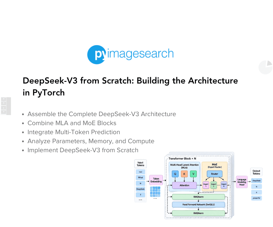
In this lesson, we will focus on assembling the full DeepSeek-V3 architecture. This is where theory and implementation converge: integrating RoPE, MLA, MoE, and MTP into a cohesive model that reflects the design principles of DeepSeek-V3. We will walk through how these components interact, the structural choices that make them synergize effectively, and the practical considerations for building a scalable, efficient language model. By the end, you will have a complete architecture blueprint, ready for the final lesson in the series, where we will implement the DeepSeek trainer and bring the model to life through training.

This lesson is the 5th in the 6-part series on Building DeepSeek-V3 from Scratch:

1. DeepSeek-V3 Model: Theory, Config, and Rotary Positional Embeddings
2. Build DeepSeek-V3: Multi-Head Latent Attention (MLA) Architecture
3. DeepSeek-V3 from Scratch: Mixture of Experts (MoE)
4. Autoregressive Model Limits and Multi-Token Prediction in DeepSeek-V3
5. DeepSeek-V3 from Scratch: Building the Architecture in PyTorch (this tutorial)
6. Lesson 6

To learn about DeepSeek-V3 and build it from scratch, just keep reading.

---

The Transformer Block: Combining MLA and MoE

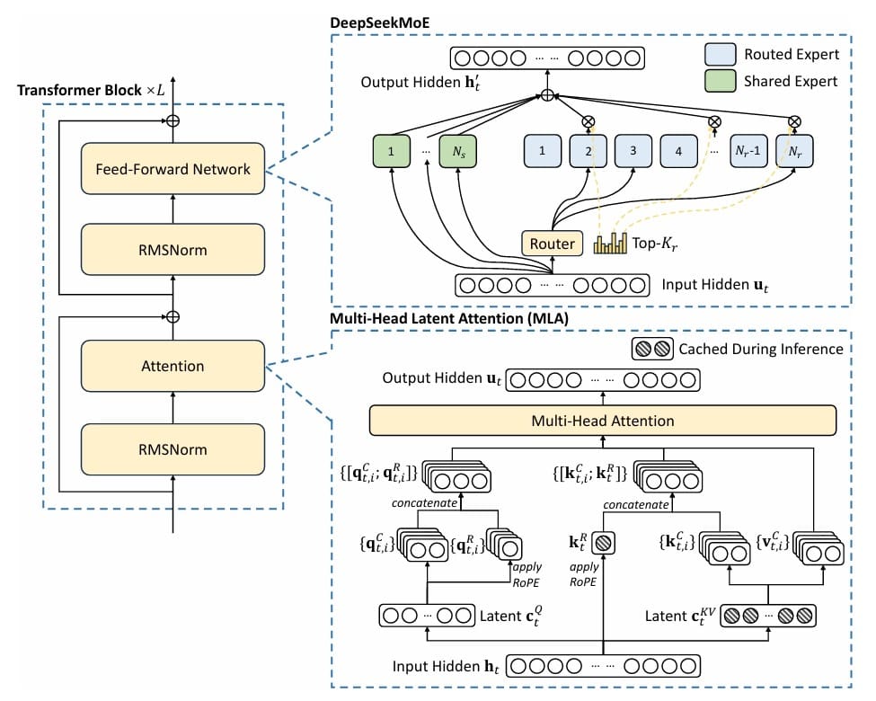
Now that we have our sophisticated components, we need to integrate them into the classic transformer architecture. A DeepSeek transformer block follows the pre-norm residual pattern:

This is the pre-layer normalization (Pre-LN) variant used in modern transformers. The residual connections allow gradients to flow directly through the network during backpropagation, addressing the vanishing gradient problem in deep networks. The layer norms stabilize the activations before they enter the attention or MoE layers.

Mathematically, each block implements a function

where is the layer index. The full model is a composition of such blocks:

where denotes the sum of the token and position embeddings. Each layer refines the representations, with early layers typically learning syntax and surface patterns while deeper layers learn semantics and abstract concepts.

---

The Complete Model: From Tokens to Logits

The full DeepSeek model architecture (Figure 1) consists of:

• Token Embedding: maps token identifiers (IDs) to dense vectors
• Position Embedding: provides positional information
• Input Dropout: Regularization applied to embedded representations
• Transformer Blocks: blocks combining MLA and MoE with layer normalization
• Final Layer Norm: Stabilizes representations before output projection
• Language Modeling Head: Projects to the vocabulary:
• Multi-Token Prediction Heads: Optional heads for future token prediction

The forward pass computes:

where contains the token indices and denotes the position indices.

---

Weight Tying: Sharing Token Embeddings and Output Weights

An important optimization is weight tying between the token embedding matrix and the language modeling head:

This reduces parameters significantly (for our vocabulary of 50,259 and embedding dimension of 256, we save approximately 12.9 million parameters) and often improves performance. The intuition is elegant: if token has embedding vector , then the similarity measures how much the hidden representation aligns with token . This is exactly what we want for predicting that token.

Mathematically, weight tying implements a form of parameter sharing that encourages the input and output spaces to be aligned. The embedding space becomes jointly optimized for both encoding tokens into context and decoding context into tokens.

---

Multi-Token Prediction Integration

During training, after computing the main hidden states , we process them through MTP heads:

Each head takes the previous layer’s output and the embedding of the next actual token (ground truth during training), processes them through its mini-transformer, and projects the result to the vocabulary. We compute losses for all predictions and combine them:

where and are cross-entropy losses, are MTP weights, and is the MoE load-balancing loss with coefficient .

---

Implementing the DeepSeek-V3 Architecture in PyTorch

Let us implement the full architecture:

class DeepSeekBlock(nn.Module):
    """DeepSeek transformer block with MLA and MoE"""

    def __init__(self, config: DeepSeekConfig):
        super().__init__()
        self.config = config

        # Layer norms (pre-norm architecture)
        self.ln1 = nn.LayerNorm(config.n_embd, bias=config.bias)
        self.ln2 = nn.LayerNorm(config.n_embd, bias=config.bias)

        # Attention - MLA
        self.attn = MultiheadLatentAttention(config)

        # MoE feedforward
        self.moe = MixtureOfExperts(config)

Lines 1-16: Block Structure: The DeepSeekBlock class encapsulates a single transformer layer. We use 2 layer norms (ln1 and ln2) for the pre-norm architecture, which normalizes inputs before they enter the attention and feedforward (MoE) sublayers. This has proven more stable for training than post-norm architectures. The block contains our custom MLA mechanism and MoE feedforward layer, both of which we have already implemented.

    def forward(self, x: torch.Tensor, attention_mask: Optional[torch.Tensor] = None):
        # Attention with residual connection
        x = x + self.attn(self.ln1(x), attention_mask)

        # MoE with residual connection
        moe_output, router_logits  = self.moe(self.ln2(x))
        x = x + moe_output
        return x, router_logits

Lines 18-25: Forward Pass with Residual Connections: The forward method implements the classic “attention then feedforward” pattern with residual connections. First, we normalize the input, pass it through attention, and add it back to the original input (residual connection). Then we normalize again, pass through MoE, and add another residual. Importantly, we return both the output and router_logits from MoE. These router logits are needed for computing auxiliary losses during training. The residual connections are crucial: they allow gradients to flow directly through the network, helping mitigate vanishing gradients in deep models.

class DeepSeek(nn.Module):
    """Complete DeepSeek model for children's story generation"""

    def __init__(self, config: DeepSeekConfig):
        super().__init__()
        assert isinstance(config, DeepSeekConfig)
        self.config = config

        # Embeddings and transformer blocks
        self.transformer = nn.ModuleDict(dict(
            wte=nn.Embedding(config.vocab_size, config.n_embd),
            wpe=nn.Embedding(config.block_size, config.n_embd),
            drop=nn.Dropout(config.dropout),
            h=nn.ModuleList([DeepSeekBlock(config) for _ in range(config.n_layer)]),
            ln_f=nn.LayerNorm(config.n_embd, bias=config.bias),
        ))

        # Output heads
        self.lm_head = nn.Linear(config.n_embd, config.vocab_size, bias=False)

        # Multi-Token Prediction heads
        if config.multi_token_predict > 0:
            self.mtp_heads = nn.ModuleList([
                MultiTokenPredictionHead(config, depth)
                for depth in range(1, config.multi_token_predict + 1)
            ])
        else:
            self.mtp_heads = None

        # Weight tying (share embeddings and output projection)
        self.transformer.wte.weight = self.lm_head.weight

        # Initialize weights
        self.apply(self._init_weights)

        # Special initialization for residual projections
        for pn, p in self.named_parameters():
            if pn.endswith(('o_proj.weight', 'down_proj.weight')):
                nn.init.normal_(p, mean=0.0, std=0.02 / math.sqrt(2 * config.n_layer))

Lines 27-42: Model Initialization: The DeepSeek class constructor sets up the complete model architecture. We use an nn.ModuleDict to organize the transformer components: wte for token embeddings, wpe for positional embeddings, drop for input dropout, h as a list of transformer blocks, and ln_f for the final layer norm. This organization makes the model structure clear and allows easy access to each component.

Lines 45-57: Output Heads and Weight Tying: We create the language modeling head (lm_head) that projects from the hidden dimension to the vocabulary size. If multi-token prediction is enabled, we create a list of MTP heads, one for each future depth. The crucial line self.transformer.wte.weight = self.lm_head.weight implements weight tying: the same weight matrix is used for both embedding tokens and predicting them. This reduces parameters and improves training.

Lines 62-65: Special Initialization for Residual Projections: The special initialization targets 2 types of output projections that feed into residual additions: o_proj in Multihead Latent Attention and down_proj in each SwiGLU expert. It scales their initialization by to account for the accumulation of residual connections through layers, helping prevent activation explosion.

def _init_weights(self, module):
        """Initialize model weights"""
        if isinstance(module, nn.Linear):
            nn.init.normal_(module.weight, mean=0.0, std=0.02)
            if module.bias is not None:
                nn.init.zeros_(module.bias)
        elif isinstance(module, nn.Embedding):
            nn.init.normal_(module.weight, mean=0.0, std=0.02)
        elif isinstance(module, nn.LayerNorm):
            nn.init.ones_(module.weight)
            if module.bias is not None:
                nn.init.zeros_(module.bias)

Lines 66-77: Weight Initialization: The _init_weights method implements careful initialization following best practices. Linear layers and embeddings use normal initialization with a standard deviation of 0.02. Layer normalization weights are initialized to 1, and their biases are initialized to 0 when present.

       def forward(self, input_ids: torch.Tensor, targets: Optional[torch.Tensor] = None, attention_mask: Optional[torch.Tensor] = None, **kwargs):
        """Forward pass with Multi-Token Prediction

        Main prediction: h[i] predicts token[i+1]
        MTP heads: Each depth d predicts token[i+d+1] using h[i] and embed[i+d]
        """
        device = input_ids.device
        batch_size, seq_len = input_ids.size()
        assert seq_len <= self.config.block_size

        # Get embeddings
        pos = torch.arange(0, seq_len, dtype=torch.long, device=device)
        tok_emb = self.transformer.wte(input_ids)
        pos_emb = self.transformer.wpe(pos)
        x = self.transformer.drop(tok_emb + pos_emb)
       
        # Forward through transformer blocks
        router_logits_list = []
        for block in self.transformer.h:
            x, router_logits = block(x, attention_mask=attention_mask)
            router_logits_list.append(router_logits)

        # Final layer norm
        x = self.transformer.ln_f(x)  # [B, seq_len, n_embd]
 

Lines 79-102: Forward Pass – Embeddings and Blocks: The forward method implements the complete forward pass. We first get token and position embeddings, sum them, and apply dropout. Then we iterate through all transformer blocks, collecting router logits from each MoE layer (needed for auxiliary losses). Finally, we apply the final layer norm. The hidden states x now encode the full context for each position. The forward signature also accepts an optional attention_mask of shape [B, T], which marks real tokens with 1 and padding with 0. Here, B is the batch size and T is the sequence length. We thread this mask down into every transformer block so that Multihead Latent Attention can exclude padded key positions from its attention scores.

        # Main language modeling head
        main_logits = self.lm_head(x)
        main_loss = None

        if targets is not None:
            # Compute main loss (standard next-token prediction)
            # Shift: h[i] predicts target[i+1]
            # main_logits[:, :-1, :] are predictions from h[0] to h[seq_len-2]
            # targets[:, 1:] are actual tokens at positions [1] to [seq_len-1]
            shift_logits = main_logits[:, :-1, :].contiguous()  # [B, seq_len-1, vocab_size]
            shift_targets = targets[:, 1:].contiguous()     # [B, seq_len-1]

            main_loss = F.cross_entropy(
                    shift_logits.view(-1, shift_logits.size(-1)),
                    shift_targets.view(-1),
                    ignore_index=-100
                )

Lines 105-120: Main Loss Computation: For training (when targets are provided), we compute the standard language modeling loss. We shift logits and targets by 1 position because we are predicting the next token: main_logits[:, i] should predict targets[:, i+1]. The cross-entropy loss with ignore_index=-100 excludes target positions labeled -100, including padding positions if they use that label. This is the base training objective.

             # Multi-Token Prediction
            mtp_loss = None
            if self.mtp_heads is not None:
                mtp_losses = []
                current_hidden = x

                for depth, mtp_head in enumerate(self.mtp_heads, 1):
                    # Check if we have enough future tokens
                    if seq_len > depth:
                        # Get future token embeddings
                        future_indices = input_ids[:, depth:]
                        future_embeds = self.transformer.wte(future_indices)

                        # Pad or truncate to match current_hidden sequence length
                        if future_embeds.size(1) < current_hidden.size(1):
                            pad_size = current_hidden.size(1) - future_embeds.size(1)
                            padding = torch.zeros(
                                batch_size, pad_size, self.config.n_embd,
                                device=device, dtype=future_embeds.dtype
                            )
                            future_embeds = torch.cat([future_embeds, padding], dim=1)
                        elif future_embeds.size(1) > current_hidden.size(1):
                            future_embeds = future_embeds[:, :current_hidden.size(1)]

                        # Process through MTP head
                        current_hidden = mtp_head(current_hidden, future_embeds, attention_mask=attention_mask)
                        mtp_logits = self.lm_head(current_hidden)

                        # Compute loss for this depth
                        # mtp_logits[:, i] predicts target[i + depth + 1]
                        if seq_len > depth + 1:
                            shift_logits = mtp_logits[:, :-(depth+1), :].contiguous()
                            shift_labels = targets[:, depth+1:].contiguous()

                            if shift_labels.numel() > 0:
                                mtp_loss_single = F.cross_entropy(
                                    shift_logits.view(-1, shift_logits.size(-1)),
                                    shift_labels.view(-1),
                                    ignore_index=-100
                                )
                                mtp_losses.append(mtp_loss_single)

                # Average MTP losses
                if mtp_losses:
                    mtp_loss = torch.stack(mtp_losses).mean()

Lines 123-166: Multi-Token Prediction: If MTP heads exist, we compute additional losses for future token prediction. For each depth, we get embeddings of the future tokens, process them through the MTP head combined with current hidden states, and compute predictions. The key insight: each MTP head receives both the context (via current_hidden) and embeddings of future ground-truth tokens (via future_embeds). We carefully handle sequence length issues by padding or truncating, and we pass the attention_mask into each MTP head, since every head runs its own mini-transformer (MLA and MoE) and must ignore padded positions for the same reason the main blocks do. All MTP losses are averaged and weighted by 0.3 relative to the main loss.

            # Add MoE auxiliary loss
            aux_loss = 0.0
            if router_logits_list:
                for i, block in enumerate(self.transformer.h):
                    aux_loss += block.moe._complementary_sequence_aux_loss(router_logits_list[i], seq_mask=attention_mask)
                aux_loss = aux_loss / len(router_logits_list)

            # Combine losses
            total_loss = main_loss
            if mtp_loss is not None:
                total_loss = total_loss + 0.3 * mtp_loss  # Weight MTP loss
           
            total_loss = total_loss + self.config.aux_loss_weight * aux_loss

            return main_logits, total_loss
        else:
            # Inference mode
            logits = self.lm_head(x[:, [-1], :])
            return logits, None

Lines 167-181: Auxiliary Loss and Combination: We compute the complementary sequence-wise auxiliary loss from all MoE layers and average across layers. This encourages load balancing among experts. We pass seq_mask=attention_mask so that padded positions are excluded when measuring expert load; without it, padding would be counted as real tokens and would skew the balancing signal toward whichever experts happen to absorb it. The total loss combines the main prediction loss, MTP loss (if enabled), and auxiliary loss (weighted by self.config.aux_loss_weight). This multi-objective training improves model quality while maintaining computational efficiency.

Lines 184 and 185: Inference Mode: When no targets are provided (inference), we simply compute logits for the last position and return them. This is used during generation when we predict 1 token at a time. No MTP heads are used during inference. They have already served their purpose in improving training.

    @torch.no_grad()
    def generate(self, input_ids: torch.Tensor, max_new_tokens: int = 100,
                 temperature: float = 1.0, top_k: Optional[int] = None):
        """Generate text autoregressively"""
        for _ in range(max_new_tokens):
            # Crop to context window
            idx_cond = input_ids if input_ids.size(1) <= self.config.block_size else input_ids[:, -self.config.block_size:]

            # Forward pass (no targets, so inference mode)
            logits, _ = self(idx_cond)  # [B, 1, vocab_size]
            logits = logits[:, -1, :] / temperature  # [B, vocab_size]

            # Apply top-k filtering
            if top_k is not None:
                v, _ = torch.topk(logits, min(top_k, logits.size(-1)))
                logits[logits < v[:, [-1]]] = -float('Inf')

            # Sample next token
            probs = F.softmax(logits, dim=-1)
            idx_next = torch.multinomial(probs, num_samples=1)  # [B, 1]
            input_ids = torch.cat((input_ids, idx_next), dim=1)

        return input_ids

Lines 186-208: Autoregressive Generation: The generate method implements text generation. For each new token, we crop the input to the context window (if it has grown too large), compute logits, apply temperature scaling and top-k filtering, sample from the distribution, and append to the input. This continues for max_new_tokens iterations. Temperature controls randomness (lower values make sampling more deterministic), while top-k prevents sampling very unlikely tokens that might break coherence.

---

Architectural Design Patterns

Several design patterns in our architecture are worth highlighting:

Pre-Norm vs Post-Norm: We use pre-normalization (normalization before the sublayer) rather than post-normalization (normalization after the sublayer). Research has shown pre-norm is more stable for training deep networks, though post-norm can sometimes achieve slightly better performance if training succeeds. The stability-performance tradeoff generally favors pre-norm for modern large models.

Residual Connection Placement: Every sublayer (attention, MoE) has a residual connection. This is crucial for gradient flow in deep networks. Without residuals, gradients would have to flow through many sequential transformations, leading to vanishing or exploding gradients. With residuals, gradients have a direct path to earlier layers.

Dropout Placement: We apply dropout in 3 places: input embeddings, within attention and MoE sublayers (implemented in those modules), and in MTP heads. This multi-level dropout provides regularization at different stages of computation. Too much dropout can hurt performance; too little can cause overfitting. Our 0.1 rate is moderate.

Weight Tying: Sharing weights between embeddings and output projection is an elegant constraint that reduces parameters and often helps. The theoretical justification is that both mappings operate in the same semantic space: the space of token meanings.

---

Parameter Count Analysis

Let us analyze where parameters are allocated:

• Embeddings: parameters
• Position Embeddings: parameters
• Per Layer (MLA and MoE): Approximately 2-3 million parameters
• Total (6 layers): Approximately 30-35 million parameters
• MTP Heads: An additional 2-3 million parameters per head

Most parameters are in the embeddings and the transformer blocks. The MLA compression reduces attention parameters compared to standard transformers, while MoE increases feedforward parameters. The balance results in a model that is larger than a standard transformer of the same compute cost, but not proportionally to the number of experts.

---

Memory and Computation Footprint

During training, memory usage includes:

• Model Parameters: Approximately 30-35 million parameters at 4 bytes each require 120-140 megabytes (MB) in 32-bit floating-point format (FP32)
• Gradients: Require the same memory as the parameters: 120-140 MB
• Optimizer States: Require twice the parameter memory with AdamW: 240-280 MB
• Activations: Memory usage depends on batch size and sequence length
• Key-Value (KV) Cache: Not needed during training

Total training memory is roughly 500-600 MB plus activations. For a batch size of 4 and sequence length of 1024, activations add approximately 200-300 MB, giving us approximately 800 MB total. This fits comfortably on modern graphics processing units (GPUs).

During inference, we do not need gradients or optimizer states, and we can use 16-bit floating-point format (FP16), roughly halving memory. This implementation does not use a KV cache; it recomputes the context during each generation step.

With all components assembled, we have a complete, working DeepSeek-V3 model. It combines 4 innovations into a coherent architecture: configuration management with RoPE, MLA for efficient attention, MoE for sparse scaling, and MTP for richer training. In the next lesson, we will train this model on real data and see it generate text.

---

---

Summary

In this 5th lesson of our DeepSeek-V3 From Scratch series, we bring everything together by assembling the full DeepSeek-V3 architecture. We start with an overview of how the different components (MLA, MoE, and RoPE) fit into the broader design, and then move into the construction of the transformer block, where Multihead Latent Attention and Mixture of Experts are combined to form the model’s core computational unit. This sets the stage for understanding how the complete model processes information, from raw tokens all the way to logits.

We then explore key architectural innovations such as weight tying, which shares weights between the token embedding layer and the language modeling head, and multi-token prediction integration, which improves efficiency and predictive power. These design choices are not just theoretical. They directly impact how the model learns and generalizes. The implementation section walks us through building the complete DeepSeek model step by step, showing how each piece connects seamlessly into a unified system.

Finally, we analyze the architectural design patterns, parameter counts, and the memory and computation footprint of DeepSeek-V3. This helps us evaluate trade-offs between scalability and efficiency, and understand how the model balances complexity with performance. By the end of this lesson, we have not only assembled the architecture but also gained insight into the design decisions that make DeepSeek-V3 both powerful and practical.

---

Citation Information

Mangla, P. “DeepSeek-V3 from Scratch: Building the Architecture in PyTorch,” PyImageSearch, S. Huot, A. Sharma, and P. Thakur, eds., 2026, https://pyimg.co/36gvk

@incollection{Mangla_2026_deepseek-v3-from-scratch-building-architecture-in-pytorch,
  author = {Puneet Mangla},
  title = {{DeepSeek-V3 from Scratch: Building the Architecture in PyTorch}},
  booktitle = {PyImageSearch},
  editor = {Susan Huot and Aditya Sharma and Piyush Thakur},
  year = {2026},
  url = {https://pyimg.co/36gvk},
}

---

To download the source code to this post (and be notified when future tutorials are published here on PyImageSearch), simply enter your email address in the form below!