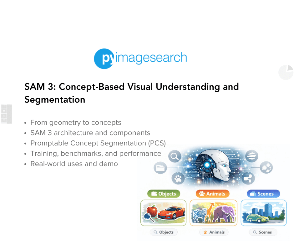
SAM 3: Concept-Based Visual Understanding and Segmentation

---

---

SAM 3: Concept-Based Visual Understanding and Segmentation

In this tutorial, we introduce Segment Anything Model 3 (SAM 3), the shift from geometric promptable segmentation to open-vocabulary concept segmentation, and why that matters.

First, we summarize the model family’s evolution (SAM-1 → SAM-2 → SAM-3), outline the new Perception Encoder + DETR detector + Presence Head + streaming tracker architecture, and describe the SA-Co data engine that enabled large-scale concept supervision.

Finally, we set up the development environment and show single-prompt examples to demonstrate the model’s basic image segmentation workflow.

By the end of this tutorial, we’ll have a solid understanding of what makes SAM 3 revolutionary and how to perform basic concept-driven segmentation using text prompts.

This lesson is the 1st of a 4-part series on SAM 3:

1. SAM 3: Concept-Based Visual Understanding and Segmentation (this tutorial)
2. Lesson 2
3. Lesson 3
4. Lesson 4

To learn about SAM 3 and how to perform concept segmentation on images using text prompts, just keep reading.

---

The release of the Segment Anything Model 3 (SAM 3) marks a definitive transition in computer vision, shifting the focus from purely geometric object localization to a sophisticated, concept-driven understanding of visual scenes.

Developed by Meta AI, SAM 3 is described as the first unified foundation model capable of detecting, segmenting, and tracking all instances of an open-vocabulary concept across images and videos via natural language prompts or visual exemplars.

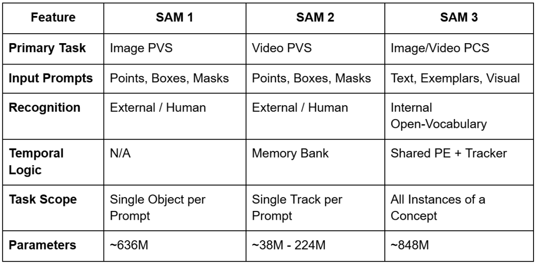
While its predecessors (i.e., SAM 1 and SAM 2) established the paradigm of Promptable Visual Segmentation (PVS) by allowing users to define objects via points, boxes, or masks, they remained semantically agnostic. As a result, they essentially functioned as high-precision geometric tools.

SAM 3 transcends this limitation by introducing Promptable Concept Segmentation (PCS). This task internalizes semantic recognition and enables the model to “understand” user-provided noun phrases (NPs).

This transformation from a geometric segmenter to a vision foundation model is facilitated by a massive new dataset, SA-Co (Segment Anything with Concepts), and a novel architectural design that decouples recognition from localization.

---

The Evolution of Segment Anything: From Geometry to Concepts

The trajectory of the Segment Anything project reflects a broader trend in artificial intelligence toward multi-modal unification and zero-shot generalization.

SAM 1, released in early 2023, introduced the concept of a promptable foundation model for image segmentation, capable of zero-shot generalization to unseen domains by using simple spatial prompts.

Released in 2024, SAM 2 extended this capability to the temporal domain by utilizing a memory bank architecture to track single objects across video frames with high temporal consistency.

However, both models suffered from a common bottleneck: they required an external system or a human operator to tell them where an object was before they could determine its extent.

SAM 3 addresses this foundational gap by integrating an open-vocabulary detector directly into the segmentation and tracking pipeline. This integration allows the model to resolve “what” is in the image, effectively turning segmentation into a query-based search interface.

For example, whereas SAM 2 required users to click on every car in a parking lot to segment them, SAM 3 can accept the text prompt “cars” and instantly return masks and unique identifiers for each individual car in the scene. This evolution is summarized in the following comparison of the 3 model generations.

---

Core Model Architecture and Technical Components

The architecture of SAM 3 represents a fundamental departure from previous models, moving to a unified, dual encoder-decoder transformer system.

The model comprises approximately 848 million parameters (depending on configuration), a significant scale-up from the largest SAM 2 variants, reflecting the increased complexity of the open-vocabulary recognition task.

These parameters are distributed across 3 main architectural pillars:

• shared Perception Encoder (PE)
• DETR-based detector
• memory-based tracker

---

The Perception Encoder (PE) and Vision Backbone

Central to SAM 3’s design is the Perception Encoder (PE), a vision backbone that is shared between the image-level detector and the video-level tracker.

This shared design is critical for ensuring that visual features are processed consistently across both static and temporal domains, minimizing task interference and maximizing data scaling efficiency.

Unlike SAM 2, which utilized the Hiera architecture, SAM 3 employs a ViT-style perception encoder that is more easily aligned with the semantic embeddings of the text encoder.

The vision encoder accounts for approximately 450 million parameters and is designed to handle high-resolution inputs (often scaled to 1024 or 1008 pixels) to preserve the spatial detail necessary for precise mask generation.

The encoder’s output embeddings, typically of size with 1024 channels, are passed to a fusion encoder that conditions them based on the provided prompt tokens.

---

The Open-Vocabulary Text and Exemplar Encoders

To facilitate Promptable Concept Segmentation, SAM 3 integrates a sophisticated text encoder with approximately 300 million parameters. This encoder processes noun phrases using a specialized Byte Pair Encoding (BPE) vocabulary, allowing it to handle a vast range of descriptive terms. When a user provides a text prompt, the encoder generates linguistic embeddings that are treated as “prompt tokens”.

In addition to text, SAM 3 supports image exemplars — visual crops of target objects provided by the user. These exemplars are processed by a dedicated exemplar encoder that extracts visual features to define the target concept.

This multi-modal prompt interface allows the fusion encoder to jointly process linguistic and visual cues, creating a unified concept embedding that tells the model exactly what to search for in the image.

---

The DETR-Based Detector and Presence Head

The detection component of SAM 3 is based on the DEtection TRansformer (DETR) framework, which utilizes learned object queries to interact with the conditioned image features.

In a standard DETR architecture, queries are responsible for both classifying an object and determining its location. However, in open-vocabulary scenarios, this often leads to “phantom detections.” There are false positives where the model localizes background noise because it lacks a global understanding of whether the requested concept even exists in the scene.

To solve this, SAM 3 introduces the Presence Head, a novel architectural innovation that decouples recognition from localization. The Presence Head utilizes a learned global token that attends to the entire image context and predicts a single scalar “presence score” () between 0 and 1. This score represents the probability that the prompted concept is present anywhere in the frame. The final confidence score for any individual object query is then calculated as:

where is the score produced by the individual query’s local detection. If the Presence Head determines that a “unicorn” is not in the image (score ≈ 0.01), it suppresses all local detections, preventing hallucinations across the board. This mechanism significantly improves the model’s calibration, particularly on the Image-Level Matthews Correlation Coefficient (IL_MCC) metric.

---

The Streaming Memory Tracker

For video processing, SAM 3 integrates a tracker that inherits the memory bank architecture from SAM 2 but is more tightly coupled with the detector through the shared Perception Encoder.

On each frame, the detector identifies new instances of the target concept, while the tracker propagates existing “masklets” (i.e., object-specific spatial-temporal masks) from previous frames using self- and cross-attention.

The system manages the temporal identity of objects through a matching and update stage. Propagated masks are compared with newly detected masks to ensure consistency, allowing the model to handle occlusions or objects that temporarily exit the frame.

If an object disappears behind an obstruction and later reappears, the detector provides a “fresh” detection that the tracker uses to re-establish the object’s history, preventing identity drift.

---

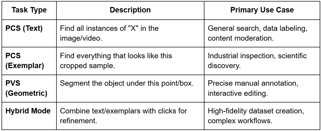
Promptable Concept Segmentation (PCS): Defining the Task

The introduction of Promptable Concept Segmentation (PCS) is the defining characteristic of SAM 3, transforming it from a tool for “segmenting that thing” to a system for “segmenting everything like that”. SAM 3 unifies several segmentation paradigms (i.e., single-image, video, interactive refinement, and concept-driven detection) under a single backbone.

---

Open-Vocabulary Noun Phrases

The model’s primary interaction mode is through text prompts. Unlike traditional object detectors that are limited to a fixed set of classes (e.g., the 80 classes in COCO), SAM 3 is open-vocabulary.

Because it has been trained on over 4 million unique noun phrases, it can understand specific descriptions (e.g., “shipping container,” “striped cat,” or “players wearing red jerseys”). This allows researchers to query datasets for specific attributes without retraining the model for every new category.

---

Image Exemplars and Hybrid Prompting

Exemplar prompting allows users to provide visual examples instead of or in addition to text.

By drawing a box around an example object, the user tells the model to “find more of these”. This is particularly useful in specialized fields where text descriptions may be ambiguous (e.g., identifying a specific type of industrial defect or a rare biological specimen).

The model also supports hybrid prompting, where a text prompt is used to narrow the search and visual prompts are used for refinement. For instance, a user can prompt for “helmets” and then use negative exemplars (boxes around bicycle helmets) to force the model to only segment construction hard hats.

This iterative refinement loop maintains the interactive “spirit” of the original SAM while scaling it to thousands of potential objects.

---

The SA-Co Data Engine and Massive Scale Dataset

The success of SAM 3 is largely driven by its training data. Meta developed an innovative data engine to create the SA-Co (Segment Anything with Concepts) dataset, which is the largest high-quality open-vocabulary segmentation dataset to date. This dataset contains approximately 5.2 million images and 52.5 thousand videos, with over 4 million unique noun phrases and 1.4 billion masks.

---

The Four-Stage Data Engine

The SA-Co data engine follows a sophisticated semi-automated feedback loop designed to maximize both diversity and accuracy.

• Media Curation: The engine curates diverse media domains, moving beyond homogeneous web data to include aerial, document, medical, and industrial imagery.
• Label Curation and AI Annotation: By leveraging a complex ontology and multimodal large language models (MLLMs) such as Llama 3.2 to serve as “AI annotators,” the system generates a massive number of unique noun phrases for the curated media.
• Quality Verification: AI annotators are deployed to check mask quality and exhaustivity. Interestingly, these AI systems are reported to be 5× faster than humans at identifying “negative prompts” (concepts not present in the scene) and 36% faster at identifying “positive prompts”.
• Human Refinement: Human annotators are used strategically, stepping in only for the most challenging examples where the AI models struggle (e.g., fine-grained boundary corrections or resolving semantic ambiguities).

---

Dataset Composition and Statistics

The resulting dataset is categorized into training and evaluation sets that cover a wide range of real-world scenarios.

• SA-Co/HQ: 5.2 million high-quality images with 4 million unique NPs.
• SA-Co/SYN: 38 million synthetic phrases with 1.4 billion masks, used for massive-scale pre-training.
• SA-Co/VIDEO: 52.5 thousand videos containing over 467,000 masklets, ensuring temporal stability.

The evaluation benchmark (SA-Co Benchmark) is particularly rigorous, containing 214,000 unique phrases across 126,000 images and videos — over 50× the concepts found in existing benchmarks (e.g., LVIS). It includes subsets (e.g., SA-Co/Gold), where each image-phrase pair is annotated by three different humans to establish a baseline for “human-level” performance.

---

Training Methodology and Optimization

The training of SAM 3 is a multi-stage process designed to stabilize the learning of diverse tasks within a single model backbone.

---

Four-Stage Training Pipeline

• Perception Encoder Pre-training: The vision backbone is pre-trained to develop a robust feature representation of the world.
• Detector Pre-training: The detector is trained on a combination of synthetic data and high-quality external datasets to establish foundational concept recognition.
• Detector Fine-tuning: The model is fine-tuned on the SA-Co/HQ dataset, where it learns to handle exhaustive instance detection, and the Presence Head is optimized using challenging negative phrases.
• Tracker Training: Finally, the tracker is trained while the vision backbone is frozen, allowing the model to learn temporal consistency without degrading the detector’s semantic precision.

---

Optimization Techniques

The training process leverages modern engineering techniques to handle the massive dataset and parameter count.

• Precision: Use of PyTorch Automatic Mixed Precision (AMP) (float16/bfloat16) to optimize memory usage on large GPUs (e.g., the H200).
• Gradient Checkpointing: Enabled for decoder cross-attention blocks to reduce memory overhead during the training of the 848M-parameter model.
• Teacher Caching: In distillation scenarios (e.g., EfficientSAM3), teacher encoder features are cached to reduce the I/O bottleneck, significantly accelerating the training of smaller “student” models.

---

Benchmarks and Performance Analysis

SAM 3 delivers a “step change” in performance, setting new state-of-the-art results across image and video segmentation tasks.

---

Zero-Shot Instance Segmentation (LVIS)

The LVIS dataset is a standard benchmark for long-tail instance segmentation. SAM 3 achieves a zero-shot mask average precision (AP) of 47.0 (or 48.8 in some reports), representing a 22% improvement over the previous best of 38.5. This indicates a vastly improved ability to recognize rare or specialized categories without explicit training on those labels.

---

The SA-Co Benchmark Results

On the new SA-Co benchmark, SAM 3 achieves a 2× performance gain over existing systems. On the Gold subset, the model reaches 88% of human-level performance, establishing it as a highly reliable tool for automated labeling.

---

Object Counting and Reasoning Benchmarks

The model’s ability to count and reason about objects is also a major highlight. In counting tasks, SAM 3 achieves an accuracy of 93.8% and a Mean Absolute Error (MAE) of just 0.12, outperforming massive models (e.g., Gemini 2.5 Pro and Qwen2-VL-72B) on precise visual grounding benchmarks.

For complex reasoning tasks (ReasonSeg), where instructions might be “the leftmost person wearing a blue vest,” SAM 3, when paired with an MLLM agent, achieves 76.0 gIoU (Generalized Intersection over Union), a 16.9% improvement over the prior state-of-the-art.

---

Real-World Applications and Industrial Impact

The versatility of SAM 3 makes it a powerful foundation for a wide range of industrial and creative applications.

---

Smart Video Editing and Content Creation

Creators can now use natural language to apply effects to specific subjects in videos. For example, a video editor can prompt “apply a sepia filter to the blue chair” or “blur the faces of all bystanders,” and the model will handle the segmentation and tracking throughout the clip. This functionality is being integrated into tools (e.g., Vibes on the Meta AI app and media editing flows on Instagram).

---

Dataset Labeling and Distillation

As SAM 3 is computationally heavy (running at 30 ms per image on an H200), its most immediate industrial impact is in scaling data annotation. Teams can use SAM 3 to automatically label millions of images with high-quality instance masks and then use this “ground truth” to train smaller, faster models like YOLO or EfficientSAM3 for real-time use on the edge (e.g., in drones or mobile apps).

---

Robotics and AR Research

SAM 3 is being utilized in Aria Gen 2 research glasses to help segment and track hands and objects from a first-person perspective. This supports contextual AR research, where a wearable assistant can recognize that a user is “holding a screwdriver” or “looking at a leaky pipe” and provide relevant holographic overlays or instructions.

---

Challenges and Future Outlook

Despite its breakthrough performance, several research frontiers remain for the Segment Anything family.

• Instruction Reasoning: While SAM 3 handles atomic concepts, it still relies on external agents (MLLMs) to interpret long-form or complex instructions. Future iterations (e.g., SAM 3-I) are working to integrate this instruction-level reasoning natively into the model.
• Efficiency and On-Device Use: The 848M parameter size restricts SAM 3 to server-side environments. The development of EfficientSAM3 through progressive hierarchical distillation is crucial for bringing concept-aware segmentation to real-time, on-device applications.
• Fine-Grained Context: In tasks involving fine-grained biological structures or context-dependent targets, text prompts can sometimes fail or provide coarse boundaries. Fine-tuning with adapters (e.g., SAM3-UNet) remains a vital research direction for adapting the foundation model to specialized scientific and medical domains.

---

Would you like immediate access to 3,457 images curated and labeled with hand gestures to train, explore, and experiment with … for free? Head over to Roboflow and get a free account to grab these hand gesture images.

---

Configuring Your Development Environment

To follow this guide, you need to have the following libraries installed on your system.

!pip install --q git+https://github.com/huggingface/transformers supervision jupyter_bbox_widget

We install the transformers library to load the SAM 3 model and processor, the supervision library for annotation, drawing, and inspection, which we use later to visualize bounding boxes and segmentation outputs. We also install jupyter_bbox_widget, which gives us an interactive widget. This widget runs inside a notebook and lets us click on the image to add points or draw bounding boxes.

We also pass the --q flag to hide installation logs. This keeps notebook output clean.

---

Need Help Configuring Your Development Environment?

All that said, are you:

• Short on time?
• Learning on your employer’s administratively locked system?
• Wanting to skip the hassle of fighting with the command line, package managers, and virtual environments?
• Ready to run the code immediately on your Windows, macOS, or Linux system?

Then join PyImageSearch University today!

Gain access to Jupyter Notebooks for this tutorial and other PyImageSearch guides pre-configured to run on Google Colab’s ecosystem right in your web browser! No installation required.

And best of all, these Jupyter Notebooks will run on Windows, macOS, and Linux!

---

Setup and Imports

Once installed, we move on to import the required libraries.

import io
import torch
import base64
import requests
import matplotlib
import numpy as np
import ipywidgets as widgets
import matplotlib.pyplot as plt

from google.colab import output
from accelerate import Accelerator
from IPython.display import display
from jupyter_bbox_widget import BBoxWidget
from PIL import Image, ImageDraw, ImageFont
from transformers import Sam3Processor, Sam3Model, Sam3TrackerProcessor, Sam3TrackerModel

We import the following:

• io: Python’s built-in module to handle in-memory image buffers later when converting PIL images to base64 format
• torch: to run the SAM 3 model, send tensors to the GPU, and work with model outputs
• base64: module to convert our images into base64 strings so that the BBox widget can display them in the notebook
• requests: library to download images directly from a URL; this keeps our workflow simple and avoids manual file uploads

We import several helper libraries.

• matplotlib.pyplot: helps us visualize masks and overlays
• numpy: gives us fast array operations
• ipywidgets: enables interactive elements inside the notebook

We import the output utility from Colab. Later, we use it to enable interactive widgets. Without this step, our bounding box widget will not render. We import Accelerator from Hugging Face to run the model efficiently on either CPU or GPU with the same code. It also simplifies device placement.

We import the display function to render images and widgets directly in notebook cells, and BBoxWidget acts as the core interactive tool that allows us to click and draw bounding boxes or points on top of an image. We use this as our prompt input system.

We also import 3 classes from Pillow:

• Image: loads RGB images
• ImageDraw: helps us draw shapes on images
• ImageFont: gives us text rendering support for overlays

Finally, we import our SAM 3 tools from transformers.

• Sam3Processor: prepares inputs for the segmentation model
• Sam3Model: performs segmentation from text and box prompts
• Sam3TrackerProcessor: prepares inputs for point-based or tracking prompts
• Sam3TrackerModel: runs point-based segmentation and masking

---

Loading the SAM 3 Model

device = "cuda" if torch.cuda.is_available() else "cpu"

processor = Sam3Processor.from_pretrained("facebook/sam3")
model = Sam3Model.from_pretrained("facebook/sam3").to(device)

First, we check if a GPU is available in the environment. If PyTorch detects CUDA (Compute Unified Device Architecture), then we use the GPU for faster inference. Otherwise, we fall back to the CPU. This check ensures our code runs efficiently on any machine (Line 1).

Next, we load the Sam3Processor. The processor is responsible for preparing all inputs before they reach the model. It handles image preprocessing, bounding box formatting, text prompts, and tensor conversion. After all, it makes our raw images compatible with the model (Line 3).

Finally, we load the Sam3Model from Hugging Face. This model takes the processed inputs and generates segmentation masks. We immediately move the model to the selected device (GPU or CPU) for inference (Line 4).

---

Downloading a Few Images

!wget -q https://media.roboflow.com/notebooks/examples/birds.jpg
!wget -q https://media.roboflow.com/notebooks/examples/traffic_jam.jpg
!wget -q https://media.roboflow.com/notebooks/examples/basketball_game.jpg
!wget -q https://media.roboflow.com/notebooks/examples/dog-2.jpeg

Here, we download a few images from the Roboflow media server using the wget command and use the -q flag to suppress output and keep the notebook clean.

---

Helper Function

This helper overlays segmentation masks, bounding boxes, labels, and confidence scores directly on top of the original image. We use it throughout the notebook to visualize model predictions.

def overlay_masks_boxes_scores(
   image,
   masks,
   boxes,
   scores,
   labels=None,
   score_threshold=0.0,
   alpha=0.5,
):
   image = image.convert("RGBA")

   masks = masks.cpu().numpy()
   boxes = boxes.cpu().numpy()
   scores = scores.cpu().numpy()

   if labels is None:
       labels = ["object"] * len(scores)

   labels = np.array(labels)

   # Score filtering
   keep = scores >= score_threshold
   masks = masks[keep]
   boxes = boxes[keep]
   scores = scores[keep]
   labels = labels[keep]

   n_instances = len(masks)
   if n_instances == 0:
       return image

   # Colormap (one color per instance)
   cmap = matplotlib.colormaps.get_cmap("rainbow").resampled(n_instances)
   colors = [
       tuple(int(c * 255) for c in cmap(i)[:3])
       for i in range(n_instances)
   ]

First, we define a function named overlay_masks_boxes_scores. It accepts the original RGB image and the model outputs: masks, boxes, and scores. We also accept optional labels, a score threshold, and a transparency factor alpha (Lines 1-9).

Next, we convert the image into RGBA format. The extra alpha channel allows us to blend masks smoothly on top of the image (Line 10). We move the tensors to the CPU and convert them to NumPy arrays. This makes them easier to manipulate and compatible with Pillow (Lines 12-14).

If the user does not provide labels, we assign a default label string to each detected object (Lines 16 and 17). We convert labels to a NumPy array so we can filter them later, along with masks and scores (Line 19). We filter out detections below the score threshold. This allows us to hide low-confidence masks and reduce clutter in the visualization (Lines 22-26). If nothing survives filtering, we return the original image unchanged (Lines 28-30).

We select a rainbow colormap and sample one unique color per detected object. We convert float values to RGB integer tuples (0-255 range) (Lines 33-37).

   # =========================
   # PASS 1: MASK OVERLAY
   # =========================
   for mask, color in zip(masks, colors):
       mask_img = Image.fromarray((mask * 255).astype(np.uint8))
       overlay = Image.new("RGBA", image.size, color + (0,))
       overlay.putalpha(mask_img.point(lambda v: int(v * alpha)))
       image = Image.alpha_composite(image, overlay)

Here, we loop through each mask-color pair. For each mask, we create a grayscale mask image, convert it into a transparent RGBA overlay, and blend it onto the original image. The alpha value controls transparency. This step adds soft, colored regions over segmented areas (Lines 42-46).

   # =========================
   # PASS 2: BOXES + LABELS
   # =========================
   draw = ImageDraw.Draw(image)

   try:
       font = ImageFont.load_default()
   except Exception:
       font = None

   for box, score, label, color in zip(boxes, scores, labels, colors):
       x1, y1, x2, y2 = map(int, box.tolist())

       # --- Bounding box (with black stroke for visibility)
       draw.rectangle([(x1, y1), (x2, y2)], outline="black", width=3)
       draw.rectangle([(x1, y1), (x2, y2)], outline=color, width=2)

       # --- Label text
       text = f"{label} | {score:.2f}"
       tb = draw.textbbox((0, 0), text, font=font)
       tw, th = tb[2] - tb[0], tb[3] - tb[1]

       # Label background
       draw.rectangle(
           [(x1, y1 - th - 4), (x1 + tw + 6, y1)],
           fill=color,
       )

       # Black label text (high contrast)
       draw.text(
           (x1 + 3, y1 - th - 2),
           text,
           fill="black",
           font=font,
       )

   return image

Here, we prepare a drawing context to overlay rectangles and text (Line 51). We attempt to load a default font. If unavailable, we fall back to no font (Lines 53-56). We loop over each object and extract its bounding box coordinates (Lines 58 and 59).

We draw two rectangles: The first one (black) improves visibility, and the second one uses the assigned object color (Lines 62 and 63). We format the label and score text, then compute the text box size (Lines 66-68). We draw a colored background rectangle behind the label text (Lines 71-74). We draw black text on top. Black text provides a strong contrast against bright overlay colors (Lines 77-82).

Finally, we return the annotated image (Line 84).

---

Promptable Concept Segmentation on Images: Single Text Prompt on a Single Image

Now, we are ready to show Promptable Concept Segmentation on images.

In this example, we segment specific visual concepts from an image using only a single text prompt.

---

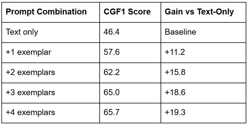
Example 1

# Load image
image_url = "http://images.cocodataset.org/val2017/000000077595.jpg"
image = Image.open(requests.get(image_url, stream=True).raw).convert("RGB")

# Segment using text prompt
inputs = processor(images=image, text="ear", return_tensors="pt").to(device)

with torch.no_grad():
   outputs = model(**inputs)

# Post-process results
results = processor.post_process_instance_segmentation(
   outputs,
   threshold=0.5,
   mask_threshold=0.5,
   target_sizes=inputs.get("original_sizes").tolist()
)[0]

print(f"Found {len(results['masks'])} objects")
# Results contain:
# - masks: Binary masks resized to original image size
# - boxes: Bounding boxes in absolute pixel coordinates (xyxy format)
# - scores: Confidence scores

First, we load a test image from the COCO (Common Objects in Context) dataset. We download it directly via URL, convert its bytes into a PIL image, and ensure it is in RGB format using Image from Pillow. This provides a standardized input for SAM 3 (Lines 2 and 3).

Next, we prepare the model inputs. We pass the image and a single text prompt — the keyword "ear". The processor handles all preprocessing steps (e.g., resizing, normalization, and token encoding). We move the final tensors to our selected device (GPU or CPU) (Line 6).

Then, we run inference. We disable gradient tracking using torch.no_grad(). This reduces memory usage and speeds up forward passes. The model returns raw segmentation outputs (Lines 8 and 9).

After inference, we convert raw model outputs into usable instance-level segmentation predictions using processor.post_process_instance_segmentation (Lines 12-17).

• We apply a threshold to filter weak detections.
• We apply mask_threshold to convert predicted logits into binary masks.
• We resize masks back to their original dimensions.

We index [0] because this output corresponds to the first (and only) image in the batch (Line 17).

We print the number of detected instance masks. Each mask corresponds to one “ear” found in the image (Line 19).

Below is the number of objects detected in the image.

Found 2 objects

Output

labels = ["ear"] * len(results["scores"])
overlay_masks_boxes_scores(
   image,
   results["masks"],
   results["boxes"],
   results["scores"],
   labels
)

Now, to visualize the output, we assign the label "ear" to each detected instance. This ensures our visualizer displays clean text overlays.

Finally, we call our visualization helper. This overlays:

• segmentation masks
• bounding boxes
• labels
• scores

directly on top of the image. The result is a clear visual map showing where SAM 3 found ears in the scene (Lines 2-8).

In Figure 1, we can see the object (ear) detected in the image.

---

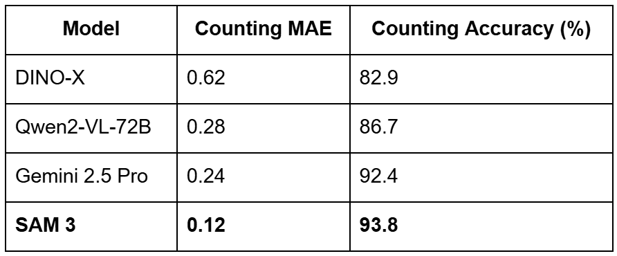
Example 2

IMAGE_PATH = '/content/birds.jpg'

# Load image
image = Image.open(IMAGE_PATH).convert("RGB")

# Segment using text prompt
inputs = processor(images=image, text="bird", return_tensors="pt").to(device)

with torch.no_grad():
   outputs = model(**inputs)

# Post-process results
results = processor.post_process_instance_segmentation(
   outputs,
   threshold=0.5,
   mask_threshold=0.5,
   target_sizes=inputs.get("original_sizes").tolist()
)[0]

print(f"Found {len(results['masks'])} objects")
# Results contain:
# - masks: Binary masks resized to original image size
# - boxes: Bounding boxes in absolute pixel coordinates (xyxy format)
# - scores: Confidence scores

This block of code is identical to the previous example. The only change is that we now load a local image (birds.jpg) instead of downloading one from COCO. We also update the segmentation prompt from "ear" to "bird".

Below is the number of objects detected in the image.

Found 45 objects

Output

labels = ["bird"] * len(results["scores"])
overlay_masks_boxes_scores(
   image,
   results["masks"],
   results["boxes"],
   results["scores"],
   labels
)

The output code remains similar to the above. The only difference is the label change from "ear" to "bird".

In Figure 2, we can see the object (bird) detected in the image.

---

Example 3

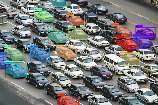
IMAGE_PATH = '/content/traffic_jam.jpg'

# Load image
image = Image.open(IMAGE_PATH).convert("RGB")

# Segment using text prompt
inputs = processor(images=image, text="taxi", return_tensors="pt").to(device)

with torch.no_grad():
   outputs = model(**inputs)

# Post-process results
results = processor.post_process_instance_segmentation(
   outputs,
   threshold=0.5,
   mask_threshold=0.5,
   target_sizes=inputs.get("original_sizes").tolist()
)[0]

print(f"Found {len(results['masks'])} objects")
# Results contain:
# - masks: Binary masks resized to original image size
# - boxes: Bounding boxes in absolute pixel coordinates (xyxy format)
# - scores: Confidence scores

This block of code is identical to the previous example. The only change is that we now load a local image (traffic_jam.jpg) instead of downloading one from COCO. We also update the segmentation prompt from "bird" to "taxi".

Below is the number of objects detected in the image.

Found 16 objects

Output

labels = ["taxi"] * len(results["scores"])
overlay_masks_boxes_scores(
   image,
   results["masks"],
   results["boxes"],
   results["scores"],
   labels
)

The output code remains similar to the above. The only difference is the change of the label from "bird" to "taxi".

In Figure 3, we can see the object (taxi) detected in the image.

---

---

Summary

In this tutorial, we explored how the release of Segment Anything Model 3 (SAM 3) represents a fundamental shift in computer vision — from geometry-driven segmentation to concept-driven visual understanding. Unlike SAM 1 and SAM 2, which relied on external cues to identify where an object is, SAM 3 internalizes semantic recognition and allows users to directly query what they want to segment using natural language or visual exemplars.

We examined how this transition is enabled by a unified architecture built around a shared Perception Encoder, an open-vocabulary DETR-based detector with a Presence Head, and a memory-based tracker for videos. We also discussed how the massive SA-Co dataset and a carefully staged training pipeline allow SAM 3 to scale to millions of concepts while maintaining strong calibration and zero-shot performance.

Through practical examples, we demonstrated how to set up SAM 3 in your development environment and implement single text prompt segmentation across various scenarios — from detecting ears on a cat to identifying birds in a flock and taxis in traffic.

In Part 2, we’ll dive deeper into advanced prompting techniques, including multi-prompt segmentation, bounding box guidance, negative prompts, and fully interactive segmentation workflows that give you pixel-perfect control over your results. Whether you’re building annotation pipelines, video editing tools, or robotics applications, Part 2 will show you how to harness SAM 3’s full potential through sophisticated prompt engineering.

---

Citation Information

Thakur, P. “SAM 3: Concept-Based Visual Understanding and Segmentation,” PyImageSearch, P. Chugh, S. Huot, G. Kudriavtsev, and A. Sharma, eds., 2026, https://pyimg.co/uming

@incollection{Thakur_2026_sam-3-concept-based-visual-understanding-and-segmentation,
  author = {Piyush Thakur},
  title = {{SAM 3: Concept-Based Visual Understanding and Segmentation}},
  booktitle = {PyImageSearch},
  editor = {Puneet Chugh and Susan Huot and Georgii Kudriavtsev and Aditya Sharma},
  year = {2026},
  url = {https://pyimg.co/uming},
}

---

To download the source code to this post (and be notified when future tutorials are published here on PyImageSearch), simply enter your email address in the form below!