Object Detection with the PaliGemma 2 Model

---

---

Object Detection with the PaliGemma 2 Model

In our previous three tutorials, we explored PaliGemma in-depth — covering its architecture, fine-tuning, and various tasks it can perform. We also built interactive applications using Gradio and deployed them on Hugging Face Spaces to make them easily accessible.

Here’s a quick recap of what we’ve learned so far:

• In our first tutorial, we fine-tuned PaliGemma using QLoRA for Visual Question Answering (VQA) to improve inference results.
• In the second tutorial, we demonstrated multiple applications, including VQA, document understanding, and image/video captioning, using Gradio.
• In the third tutorial, we deployed these Gradio apps on Hugging Face Spaces, making them readily available for users.

Now, in this final tutorial, we will explore Object Detection with the PaliGemma 2 Model — leveraging its vision-language capabilities to identify objects, generate bounding boxes, and visualize detection results interactively using the Gradio application. Let’s get started! 🚀

Note: The implementation steps remain the same for both PaliGemma 1 and PaliGemma 2 models.

This lesson is the final of a 4-part series on Vision-Language Models:

1. Fine Tune PaliGemma with QLoRA for Visual Question Answering
2. Vision-Language Model: PaliGemma for Image Description Generator and More
3. Deploy Gradio Applications on Hugging Face Spaces
4. Object Detection with the PaliGemma 2 Model (this tutorial)

To learn how to detect objects using the PaliGemma 2 model, just keep reading.

---

Introduction

Object detection is a crucial task in computer vision that involves identifying and localizing objects within an image. Traditional models like YOLO, Faster R-CNN, and DETR rely on a fixed set of object categories and require extensive supervised training on large labeled datasets. These models can only detect objects they have seen during training, making them limited in adaptability to new categories.

Vision-Language Models (VLMs) like PaliGemma offer a more flexible, text-driven approach to object detection. Instead of being restricted to a predefined set of objects, PaliGemma allows users to define what to detect dynamically using natural language prompts. This enables open-vocabulary object detection, where the model can identify objects beyond its original training set based on contextual understanding.

Unlike traditional object detection models that directly output bounding box coordinates as tensors, PaliGemma encodes detection results as structured text using special location tokens (<loc[value]>). Each detection consists of four location tokens, which represent normalized bounding box coordinates, followed by the detected object’s label.

---

How Object Detection Works in PaliGemma Models

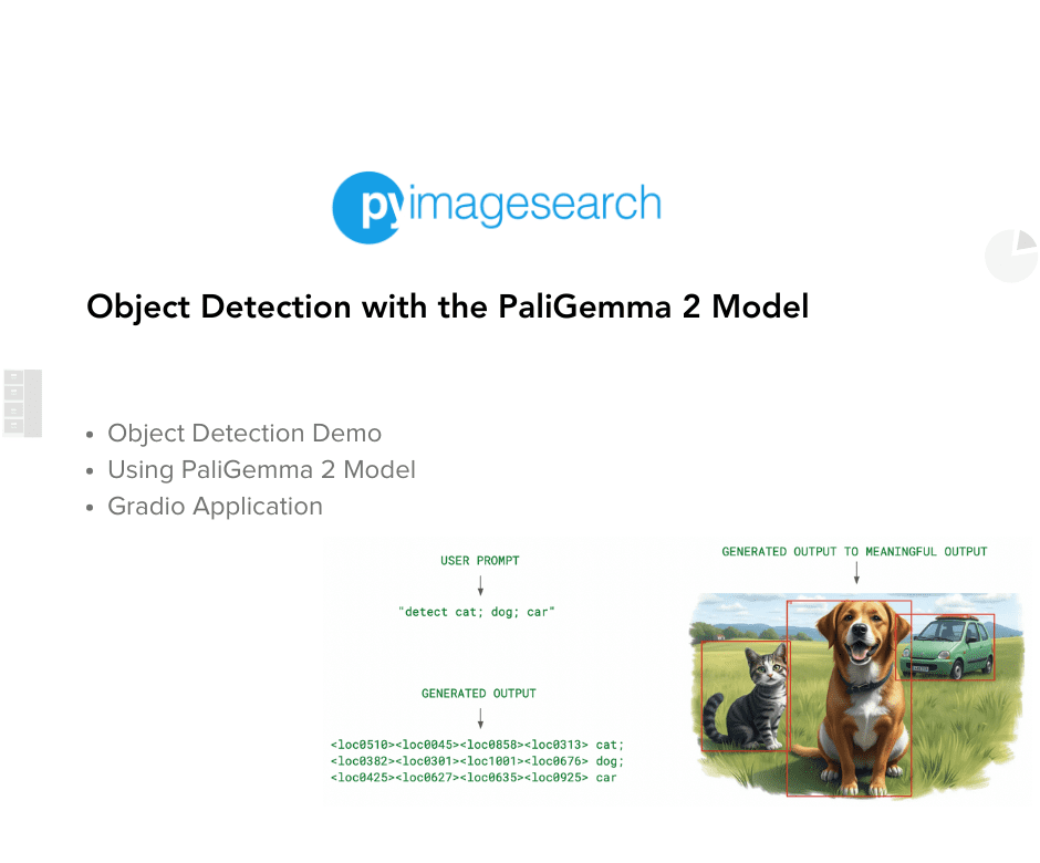
To detect objects, we provide a natural language prompt starting with a prefix detect to instruct the model to perform object detection, followed by CLASS to indicate the object to be detected. The format is:

"detect [CLASS]"

For multi-class detection, we separate object names with semicolons (;):

"detect cat; dog; car"

The model then returns an output structured as:

detect cat; dog; car

This response consists of:

• Bounding Box Coordinates: Each object is described using four <locXXXX> tokens, where each value represents a normalized coordinate between 0 and 1024. The values are structured as (y_min, x_min, y_max, x_max).
• Object Labels: The detected object’s class name follows the location tokens.
• Multi-Object Detection: PaliGemma can detect multiple objects in a single pass by returning multiple structured outputs.

---

Converting Normalized Coordinates to Pixel Values

To map the bounding box coordinates to the original image size, we:

1. Divide each extracted location value by 1024 to normalize it between 0 and 1.
2. Multiply the y values by the image height and the x values by the image width to get pixel coordinates.

By default, Google’s mix-pretrained models standardize bounding box coordinates in the (y_min, x_min, y_max, x_max) format.

This structured, text-based approach allows PaliGemma to dynamically adapt to different detection tasks, making it highly versatile for real-world applications.

In this tutorial, we will walk through a simple demo to use PaliGemma for object detection, extract structured outputs, and visualize detection results.

---

Configuring Your Development Environment

To follow this guide, you need to have the following libraries installed on your system.

!pip install -q -U transformers gradio

We install transformers to load the PaliGemma 2 model and gradio to create an interactive interface for our application.

In order to load the model from Hugging Face, we need to:

• Set up your Hugging Face Access Token
• Set up your Colab Secrets to Access Hugging Face Resources
• Grant Permission to Access the PaliGemma Model

Refer to the following blog post to complete the setup: Configure Your Hugging Face Access Token in Colab Environment

---

Need Help Configuring Your Development Environment?

All that said, are you:

• Short on time?
• Learning on your employer’s administratively locked system?
• Wanting to skip the hassle of fighting with the command line, package managers, and virtual environments?
• Ready to run the code immediately on your Windows, macOS, or Linux system?

Then join PyImageSearch University today!

Gain access to Jupyter Notebooks for this tutorial and other PyImageSearch guides pre-configured to run on Google Colab’s ecosystem right in your web browser! No installation required.

And best of all, these Jupyter Notebooks will run on Windows, macOS, and Linux!

---

Setup and Imports

import torch
import re
import cv2
import gradio as gr
from PIL import ImageDraw, Image

from transformers import AutoProcessor, PaliGemmaForConditionalGeneration

We first import torch to handle tensor computations. Next, we import the re module to work with RegEx (Regular Expressions) and cv2 for image processing. After that, we import gradio to build an interactive web interface to test our model effortlessly. Then, we import ImageDraw and Image from the PIL library to draw the bounding box in the images.

Finally, we import PaliGemmaForConditionalGeneration and AutoProcessor from the transformers library to load and process the PaliGemma model.

---

Load PaliGemma 2 Model

Once our setup is complete, we load the mixed PaliGemma 2 model, a pre-trained model designed for various tasks, including object detection.

mix_model_id = "google/paligemma2-3b-mix-224"

We first define the mix PaliGemma model (google/paligemma2-3b-mix-224) with 3b parameters and 224×224 image resolution.

mix_model = PaliGemmaForConditionalGeneration.from_pretrained(mix_model_id)

Next, we load the model using the from_pretrained method of PaliGemmaForConditionalGeneration.

mix_processor = AutoProcessor.from_pretrained(mix_model_id)

Finally, we initialize AutoProcessor to process inputs for the model.

---

Parse Multiple Locations

# Helper function to parse multiple <loc> tags and return a list of coordinate sets and labels
def parse_multiple_locations(decoded_output):
   # Regex pattern to match four <locxxxx> tags and the label at the end (e.g., 'cat')
   loc_pattern = r"<loc(\d{4})><loc(\d{4})><loc(\d{4})><loc(\d{4})>\s+(\w+)"

   matches = re.findall(loc_pattern, decoded_output)
   coords_and_labels = []

   for match in matches:
       # Extract the coordinates and label
       y1 = int(match[0]) / 1024
       x1 = int(match[1]) / 1024
       y2 = int(match[2]) / 1024
       x2 = int(match[3]) / 1024
       label = match[4]

       coords_and_labels.append({
           'label': label,
           'bbox': [y1, x1, y2, x2]
       })

   return coords_and_labels

To extract bounding box coordinates and labels from the model’s output, we define a helper function (Line 2) using Regular Expressions (RegEx).

First, we define a RegEx pattern to detect four <locxxxx> tags (Line 4), each containing four-digit coordinates, followed by a label (e.g., 'cat').

Next, we use re.findall() to find all matches in the decoded output (Line 6). We then initialize an empty list (coords_and_labels) to store the extracted bounding boxes and labels (Line 7).

After that, we iterate through the matches (Lines 9-15), extracting four coordinates and converting them from integer format (scaled by 1024) to floating-point values (normalized between 0 and 1).

Finally, we store (Lines 17-20) each label along with its corresponding bounding box coordinates.

The function returns (Line 22) a list of parsed bounding boxes and labels, ready for further processing.

---

Draw Multiple Bounding Boxes

# Helper function to draw bounding boxes and labels for all objects on the image
def draw_multiple_bounding_boxes(image, coords_and_labels):
   draw = ImageDraw.Draw(image)
   width, height = image.size

   for obj in coords_and_labels:
       # Extract the bounding box coordinates
       y1, x1, y2, x2 = obj['bbox'][0] * height, obj['bbox'][1] * width, obj['bbox'][2] * height, obj['bbox'][3] * width

       # Draw bounding box and label
       draw.rectangle([x1, y1, x2, y2], outline="red", width=3)
       draw.text((x1, y1), obj['label'], fill="red")

   return image

To visualize detected objects, we define a helper function (Line 2) that draws bounding boxes and labels on the input image.

First, we initialize ImageDraw.Draw() to allow drawing on the image (Line 3). We also extract the image dimensions (width, height) for scaling the bounding box coordinates (Line 4).

Next, we loop (Lines 6-8) through each object, convert normalized coordinates (0-1 range) into pixel values using the image dimensions (multiply the y values by the image height and the x values by the image width to get pixel coordinates), and extract the bounding box coordinates.

After that, we use draw.rectangle() to outline the detected object in red and draw.text() to label it at the top-left corner (Lines 11 and 12).

Finally, we return (Line 14) the annotated image with bounding boxes and labels, making object detection results visually interpretable.

---

Define Inference Function

# Define inference function
def process_image(image, prompt):
   # Process the image and prompt using the processor
   inputs = mix_processor(image.convert("RGB"), prompt, return_tensors="pt")

   try:
       # Generate output from the model
       output = mix_model.generate(**inputs, max_new_tokens=100)

       # Decode the output from the model
       decoded_output = mix_processor.decode(output[0], skip_special_tokens=True)

       # Extract bounding box coordinates and labels
       coords_and_labels = parse_multiple_locations(decoded_output)

       if coords_and_labels:
           # Draw bounding boxes and labels on the image
           image_with_boxes = draw_multiple_bounding_boxes(image, coords_and_labels)

           # Prepare the coordinates and labels for the UI
           labels_and_coords = "\n".join([f"Label: {obj['label']}, Coordinates: {obj['bbox']}" for obj in coords_and_labels])

           # Return image, extracted bounding boxes, and raw model output
           return image_with_boxes, decoded_output, labels_and_coords
       else:
           return "No bounding boxes detected.", "", decoded_output  # Still return raw output even if no boxes

   except IndexError as e:
       print(f"IndexError: {e}")
       return "An error occurred during processing.", "", ""

We define an inference function to process an image and a text prompt, extract bounding box information, and return an annotated image with object labels (Line 2).

First, we convert the image to RGB and process it with the prompt (Line 4) using mix_processor, ensuring compatibility with the model.

Next, we generate predictions (Line 8) using mix_model.generate, limiting the response to 100 tokens.

We decode the output (Line 11) into a human-readable format using mix_processor.decode, excluding special tokens.

Then, we extract bounding box coordinates and labels (Line 14) using the parse_multiple_locations() function defined above.

If objects are detected, we use draw_multiple_bounding_boxes() to overlay bounding boxes and labels (Lines 16-18) on the image.

We format the extracted labels and bounding box coordinates (Line 21) for easy readability.

Finally, we return the annotated image, extracted bounding boxes, and the raw model output (Line 24) for further analysis.

If no bounding boxes are detected, we still return the raw model output (Lines 25 and 26) for debugging purposes.

If an error occurs, we handle it gracefully (Lines 28-30), ensuring the function returns a consistent output format.

---

Build the Gradio Interface

We create an interactive Gradio app to detect objects in images using the Mix PaliGemma 2 model.

# Define the Gradio interface
inputs = [
   gr.Image(type="pil"),
   gr.Textbox(label="Prompt", placeholder="Enter your question")
]
outputs = [
   gr.Image(label="Output Image with Bounding Boxes"),
   gr.Textbox(label="Raw Model Output"),
   gr.Textbox(label="Bounding Box Coordinates and Labels"),
]

First, on Lines 2-5, we define the inputs:

• gr.Image: Allows users to upload an image.
• gr.Textbox: Lets users enter a prompt related to the image.

Next, on Lines 6-10, we specify the outputs:

• gr.Image: Displays the image with detected objects and bounding boxes.
• gr.Textbox: Outputs the raw model-generated text, useful for debugging.
• gr.Textbox: Shows extracted bounding box coordinates and labels.

# Create the Gradio app
demo = gr.Interface(fn=process_image, inputs=inputs, outputs=outputs, title="Object Detection with Mix PaliGemma 2 Model",
                   description="Upload an image and get object detections with bounding boxes and labels.")

# Launch the app
demo.launch(debug=True)

On Lines 13 and 14, we then create the Gradio interface using the process_image function. The title and description help users understand the app’s functionality.

Finally, on Line 17, we launch the app in debug mode using demo.launch(debug=True), enabling users to test the model by uploading images and receiving detailed detection results.

---

Generated Output

Let’s visualize the generated output.

---

First Example

In Figure 1, we can see the uploaded image and the user prompt (prefix + CLASS).

In Figure 2, we can see the output image generated with Bounding Boxes and Labels.

In Figure 3, we can see the Raw Model Output (<locXXXX> values followed by label) and extracted Bounding Box Coordinates and Labels for visualization purposes.

In Figure 4, we can see the Gradio application in action where we first uploaded an image, entered a prompt (detect cat; dog; car), and received the outputs (detected cat, dog, and car with bounding box and labels, raw model output, and extracted box coordinates and labels).

---

Second Example

In Figure 5, we can see the uploaded image and the user prompt (prefix + CLASS).

In Figure 6, we can see the output image generated with Bounding Boxes and Labels.

In Figure 7, we can see the Raw Model Output (<locXXXX> values followed by label) and extracted Bounding Box Coordinates and Labels for visualization purposes.

In Figure 8, we can see the Gradio application in action where we first uploaded an image, entered a prompt (detect cat), and received the outputs (detected cats with bounding box and labels, raw model output, and extracted box coordinates and labels).

---

---

Summary

This marks the conclusion of our 4-part series on PaliGemma. In this tutorial, we extended from PaliGemma 1 to PaliGemma 2 for object detection, leveraging its vision-language capabilities to identify and localize objects within images.

But this is just the beginning! While the PaliGemma model performs well in detecting objects, its capabilities can be further enhanced through fine-tuning for domain-specific tasks.

---

What’s Next?

Since object detection plays a crucial role in real-world applications, fine-tuning PaliGemma on specific datasets can significantly improve its accuracy and relevance.

Soon, we will kick off a 2-part series on “Object Detection with PaliGemma 2 Models”, where we will fine-tune the model for:

✅ Gaming: Detecting objects in Valorant to enhance gameplay insights.

✅ Healthcare: Detecting brain tumors in medical imaging to assist in diagnostics.

PyImageSearch University Members will also get exclusive bonus code for the following:
✅ Safety and Construction: Identifying potential hazards in construction environments for improved worker safety.

This series will showcase the versatility of PaliGemma across different industries, demonstrating how a general-purpose vision-language model can be adapted for specialized real-world tasks.

🚀 Stay tuned! The journey with PaliGemma is far from over!

---

Citation Information

Thakur, P. “Object Detection with the PaliGemma 2 Model,” PyImageSearch, P. Chugh, S. Huot, and G. Kudriavtsev, eds., 2025, https://pyimg.co/4vfxk

@incollection{Thakur_2025_Object-Detection-with-PaliGemma-2-Model,
  author = {Piyush Thakur},
  title = {{Object Detection with the PaliGemma 2 Model}},
  booktitle = {PyImageSearch},
  editor = {Puneet Chugh and Susan Huot and Georgii Kudriavtsev},
  year = {2025},
  url = {https://pyimg.co/4vfxk},
}

---

To download the source code to this post (and be notified when future tutorials are published here on PyImageSearch), simply enter your email address in the form below!